First of all, we should choose a small area to work with. A populated town or city is an obvious choice for this task. The first obstacle is that there aren't any freely available settlement polygon data in the formats we are used to. To tackle this, we can download the required data directly from OpenStreetMap. OSM offers a read-only web database for accessing its data, which is available through the Overpass API. From Overpass, we can request data through regular web requests, and the server sends the matching features as a response (Appendix 1.5). In QGIS, we can install a plugin written directly for this--QuickOSM. Therefore, our first task is to install the QuickOSM plugin as follows:

1. Open the plugin manager via Plugins | Manage and Install Plugins.
2. Type QuickOSM in the search field.
3. Click on Install plugin.

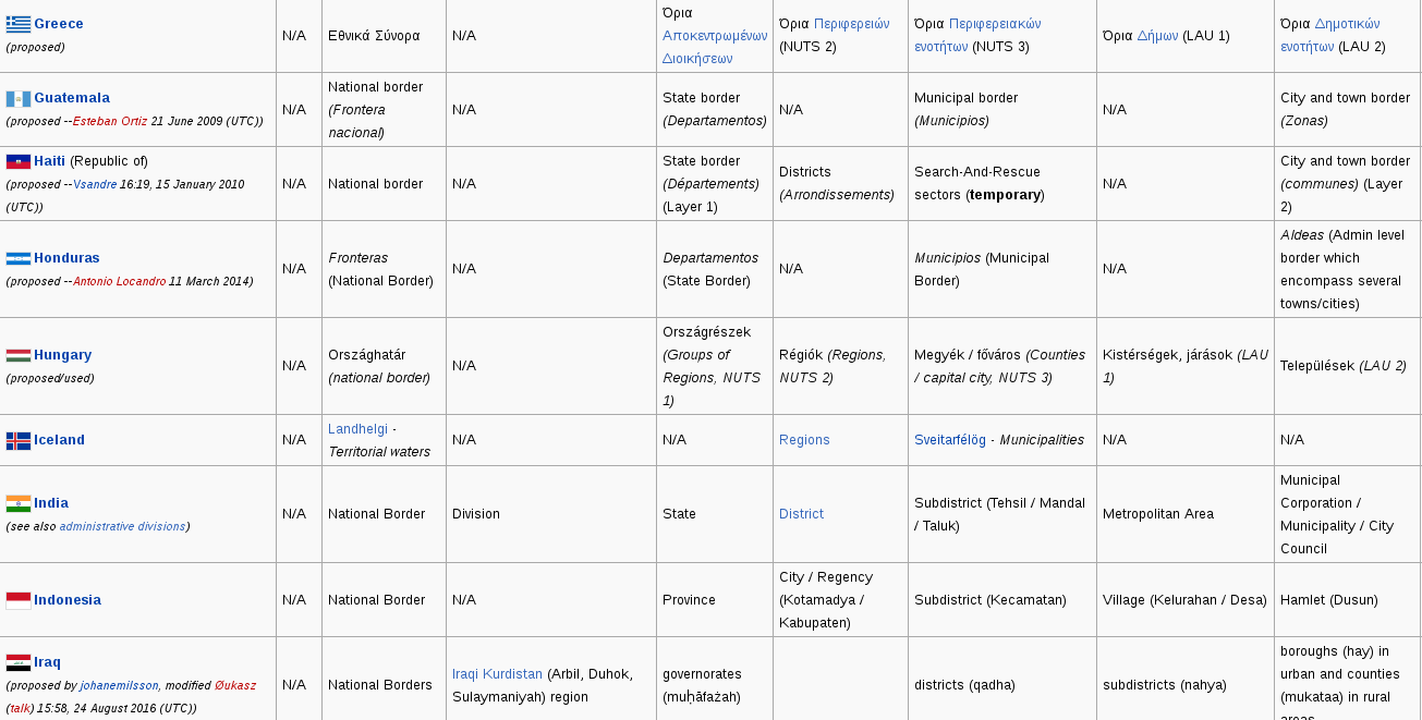
In QuickOSM, we can build Overpass requests in an interactive way. In Overpass, we can query features in a predefined area (for example, the extent of a layer), or use a name which can be geocoded to an area by OSM (for example, the name of an administrative boundary). If we open up the plugin, we can see that Overpass accepts key-value pairs according to OSM's tag specification. If we would like to request administrative boundaries, we have to use the admin_level tag as Key, and provide the appropriate level as a Value. We only need to find out the level for our country. Luckily, OSM maintains a detailed wiki about the tags it uses from where we can reach the admin_level related part at https://wiki.openstreetmap.org/wiki/Tag:boundary%3Dadministrative#admin_level:

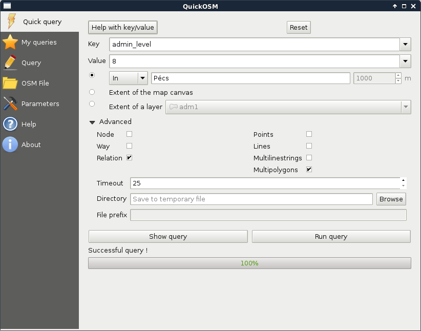
Now we can import our preferred city with the following steps:

1. Open up the QuickOSM plugin.
2. Provide admin_level as Key.
3. Find out the level that contains settlement data for your country from the aforementioned link, and provide that level as Value.

4. Check the radio box next to In, and provide the settlement's name.
5. Expand the Advanced menu.
6. Keep only the Relation and the Multipolygons boxes checked. This way, we will only request polygons from OSM.
7. Click on Run query:

As we have a smaller region for our analysis, let's generate some data. We should create points representing houses for sale with street addresses, sizes, and prices. There are various ways to achieve this. As we already did some geoprocessing, please take a little break to think about a sequence of logical steps that you would take to create these random data.

In my opinion, the easiest way is to generate the points right on the streets. We can do that as follows:

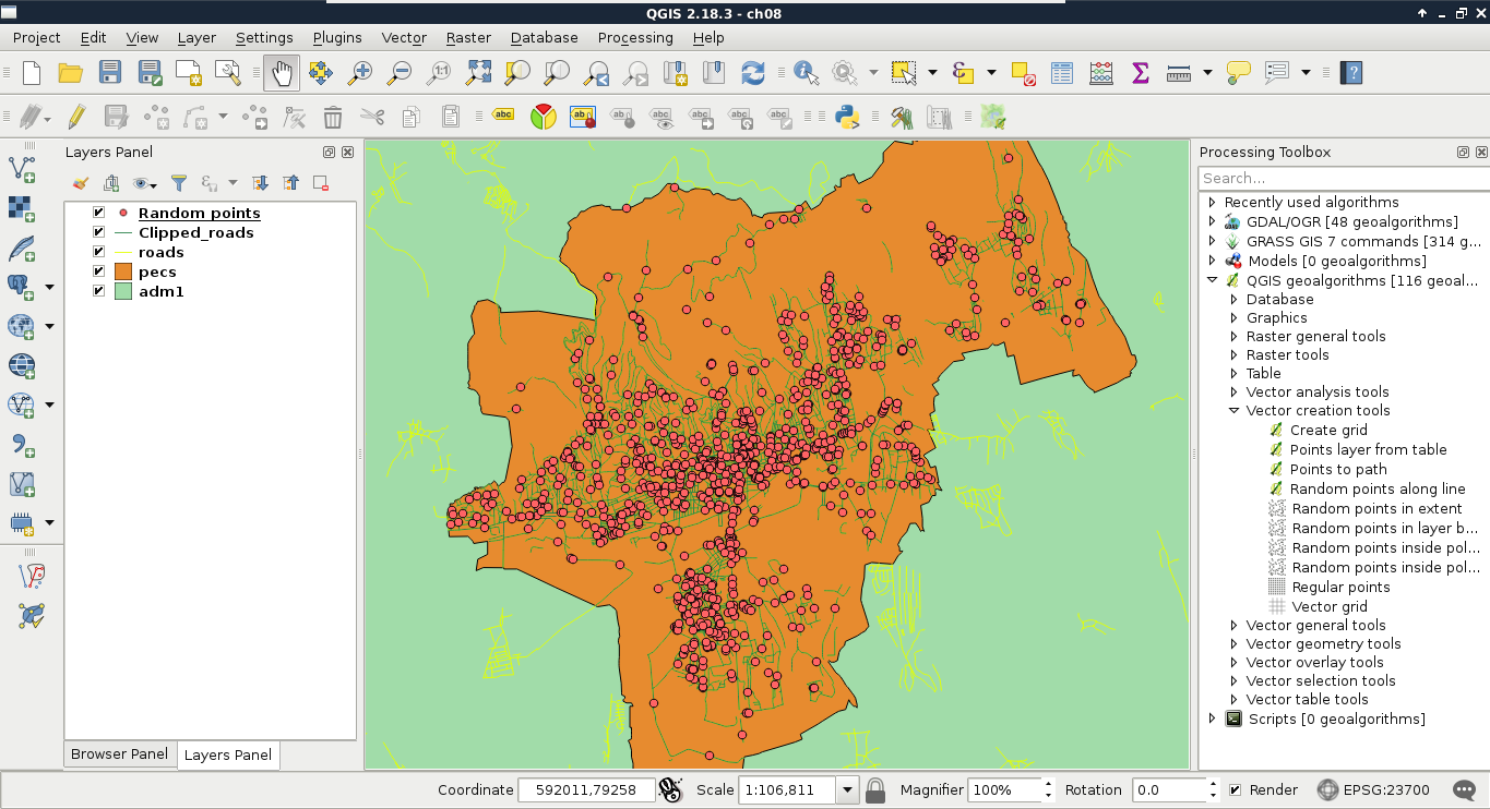
1. Load the roads layer.
2. Apply a filter on the layer which discards streets without the name attribute. Use the filter expression "name" IS NOT NULL.
3. Clip the roads layer to the town boundary. Use QGIS geoalgorithms | Vector overlay tools | Clip for this task. Save the clipped layer as a memory layer by specifying memory: as output.
4. Generate random points on the clipped road layer with QGIS geoalgorithms | Vector creation tools | Random points along line. Create at least 1,000 points, so we will always have some results. Save the points as a memory layer:

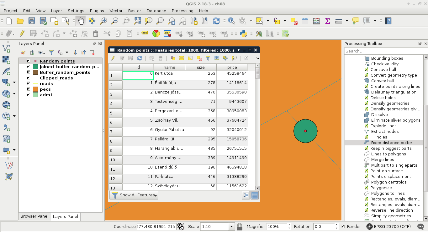
The next step is to fill our random points with data. First of all, we need to join the attributes of the roads layer to have the street names stored with our imaginary houses. The only problem is that QGIS's spatial join uses the problematic Select by location tool's algorithm. To see what I'm talking about, let's select points with it (QGIS geoalgorithms | Vector selection tools) using the intersects spatial predicate and our clipped lines layer as the intersection layer. For me, it did not select any points. One of the problems might be a precision mismatch between lines and points interpolated on them (Appendix 1.6); however, if we define a small Precision value, still only a portion of our points get selected. For me, a precision of 170 meters resulted in a full selection, where QGIS has no means to guarantee the correct street attributes get joined to the points.

What we already know about spatial queries in QGIS--checking point-polygon and line-polygon topological relationships--work well. Checking point-line relationships, on the other hand, does not. Therefore, the easiest workaround is to transform our points to polygons, join the street attributes to them, then join the polygon attributes back to the points. For this task, we can use the basic geoprocessing tool--buffer. It creates buffer zones around input features; therefore, if we supply a point layer to the tool, it creates regular polygons around them. The more segments a buffered point has, the more those polygons will resemble circles. There are two kind of buffer tools in QGIS--fixed buffer and variable buffer. The variable buffer tool creates buffer zones based on a numeric attribute field, while the fixed buffer tool creates buffer zones with a constant distance. Let's create those joins using the following steps:

1. Select the Fixed distance buffer tool from QGIS geoalgorithms | Vector geometry tools.
2. Supply the random points as the input layer, and a small value as Distance. A value of 0.1 meters should be fine. Save the result as a memory layer.
3. Use the Join attributes by location tool from QGIS geoalgorithms | Vector general tools for the first join. The target layer should be the buffered points layer, while the join layer should be the clipped roads layer. The spatial predicate is intersects. Save the result as a memory layer.
4. In this step, we can either use the same tool to join the attributes back to the random points layer, or do ourselves a favor and use a simple join. As both the tools preserved the existing attributes, we have the original IDs of our random points on the joined buffered points layer. That is, we can specify a regular join in the original random points layer's Joins tab in its Properties menu. When we add a new join, we should specify the joined buffered points layer as the Join layer, and the id field as the join and target fields. Finally, we should restrict the joined columns to the name column, as we do not need any other data from the roads layer.

5. Open the Field calculator for the random points layer. Create a new integer field named size, and use QGIS's rand function to fill it with random integers between two limits. If you would like to create sizes between 50 and 500, for example, you have to provide the expression rand(50, 500).
6. Create another integer field named price, and fill it with random numbers in a range of your liking. As I'm using my currency (HUF), I provided the expression rand(8000000, 50000000). Watch out for the Output field length value, as the upper bound should fit in the provided value.
7. Exit the edit session, and save the edits made to the points layer. Save the layer in your working folder, and remove all other intermediate data (including the clipped roads):