
Although PostGIS is one of the state-of-the-art GIS softwares for effective spatial queries, aggregating effectively can sometimes be tricky. For this reason, we will go step by step through appealing to the final criterion. First of all, we need to select the markets from our POI table. This should be easy, as we just have to chain some queries on a single column together with the logical OR operator. Or we can use a more convenient operator created for similar tasks called IN. By using IN, we can supply a collection of values to check a single column against:
    SELECT geom FROM spatial.pois p
     WHERE p.fclass IN ('supermarket', 'convenience',
     'mall', 'general');
Let's put this table in a WITH clause, and go on with counting points.
    WITH markets AS (
     SELECT geom FROM spatial.pois p
     WHERE p.fclass IN ('supermarket', 'convenience',
     'mall', 'general'));
We used some aggregating functions before, but only for the sole purpose of returning a single aggregated value for an entire table. Aggregating a single column is trivial enough for PostgreSQL not to ask for any other parameters. However, if we would like to select multiple columns while aggregating, we have to specify our intention of creating groups explicitly by using a GROUP BY expression with a selected column name. We can create a simple grouping by querying the IDs of our houses layer along with the number of geometries in our markets layer. Counting can be done by utilizing count, one of the most basic aggregating function in PostgreSQL, as follows:
    WITH markets AS (
     SELECT geom FROM spatial.pois p WHERE p.fclass IN ('supermarket',
     'convenience', 'mall', 'general'))
    SELECT h.id, count(m.geom) AS count FROM spatial.houses h,
     markets m
     GROUP BY h.id;
Now we got 1,000 results, just as many houses we have. Every row has the total count of geometries in our markets layer, as we did not supply a condition for the selection. Basically, we got the cross join of the two tables, but grouped by the IDs of our houses table. As we aggregated the number of geometries in each group, and got every possible combination, we ended up with the same number of points for every group.
Let's supply a join condition to narrow down our results:
    WITH markets AS (
     SELECT geom FROM spatial.pois p WHERE p.fclass IN ('supermarket',
     'convenience', 'mall', 'general'))
    SELECT h.id, count(m.geom) AS count FROM spatial.houses h,
     markets m
     WHERE ST_DWithin(h.geom, m.geom, 500)
     GROUP BY h.id;
By providing the condition we should be able to see a subset of our data:
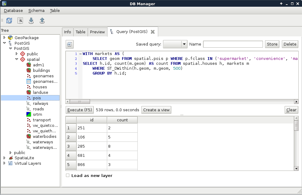
Now we get a real inner join; PostgreSQL only returned the rows matching the join conditions. That is, we got a table where every row with a geometry closer than 500 meters to a house got joined to it. From that table, PostgreSQL could easily aggregate the number of markets in the 500 meters vicinity of our houses. Note that we got back only a part of our tables, as features without markets (empty groups) got discarded. Let's take a note about that number, as we will need it later.
Before going further, let's rephrase this expression to include the INNER JOIN keywords. If we implicitly define a join, that is, separate layers in the FROM clause with commas, we can specify our join conditions in the WHERE clause. However, if we define a join explicitly, the conditions go in the ON clause:
    WITH markets AS (
     SELECT geom FROM spatial.pois p
     WHERE p.fclass IN ('supermarket', 'convenience',
     'mall', 'general'))
    SELECT h.id, count(m.geom) AS count
     FROM spatial.houses h INNER JOIN markets m
     ON ST_DWithin(h.geom, m.geom, 500)
     GROUP BY h.id;
Now we can easily change the join between our tables to an outer-left join in order to have the rest of the rows with 0 markets in their 500 meters radii:
    WITH markets AS (
     SELECT geom FROM spatial.pois p
     WHERE p.fclass IN ('supermarket', 'convenience',
     'mall', 'general'))
    SELECT h.id, count(m.geom) AS count
     FROM spatial.houses h LEFT JOIN markets m
     ON ST_DWithin(h.geom, m.geom, 500)
     GROUP BY h.id;
As the query's result shows, we have 1,000 rows, just like our houses table. Some of the rows have 0 values. However, are these results the same as the previous ones? We can do a quick validation by filtering out groups with 0 count values. If we get the same number of rows we noted previously, then we are probably on the right track. To select from groups, we cannot use a WHERE clause; we have to use a special clause designed for filtering groups--HAVING:
    WITH markets AS (
     SELECT geom FROM spatial.pois p
     WHERE p.fclass IN ('supermarket', 'convenience',
     'mall', 'general'))
    SELECT h.id, count(m.geom) AS count
     FROM spatial.houses h LEFT JOIN markets m
     ON ST_DWithin(h.geom, m.geom, 500)
     GROUP BY h.id HAVING count(m.geom) > 0;
For me, PostgreSQL returned the same number of rows; however, using LEFT JOIN and filtering with a HAVING clause slowed down the query. Before creating a CTE table along with markets from the result, we should rewrite our count table's query to its previous, faster form:
    WITH markets AS (
     SELECT geom FROM spatial.pois p
     WHERE p.fclass IN ('supermarket', 'convenience',
     'mall', 'general')),
     marketcount AS (SELECT h.id, count(m.geom) AS count
     FROM spatial.houses h, markets m
     WHERE ST_DWithin(h.geom, m.geom, 500)
     GROUP BY h.id);
Now the only thing left to do is to select the houses from our last view which have at least two markets in their vicinity:
    WITH markets AS (
     SELECT geom FROM spatial.pois p
     WHERE p.fclass IN ('supermarket', 'convenience',
     'mall', 'general')),
     marketcount AS (SELECT h.id, count(m.geom) AS count
     FROM spatial.houses h, markets m
     WHERE ST_DWithin(h.geom, m.geom, 500)
     GROUP BY h.id)
    SELECT h.* FROM spatial.vw_quietconstrainedhouses h,
     marketcount m
     WHERE h.id = m.id AND m.count >= 2;
By supplying the full query, we can see our semifinal results on our map:
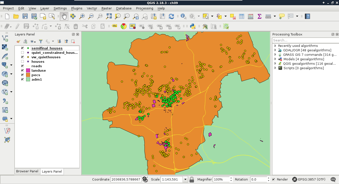
Look at that performance boost! For me, the whole analysis took about 1.3 seconds. On top of that, we can alter any parameter just by changing the view definitions. Additionally, we got the distances from the noisy places on which we can order our features. By ordering the result in a decreasing order, we can label our features according to that parameter, and show them to our customers on a map.
Finally, let's save our semifinal results as a third view:
    CREATE VIEW spatial.vw_semifinalhouses AS WITH markets AS (
     SELECT geom FROM spatial.pois p
     WHERE p.fclass IN ('supermarket', 'convenience',
     'mall', 'general')),
     marketcount AS (SELECT h.id, count(m.geom) AS count
     FROM spatial.houses h, markets m
     WHERE ST_DWithin(h.geom, m.geom, 500)
     GROUP BY h.id)
    SELECT h.* FROM spatial.vw_quietconstrainedhouses h, marketcount m
     WHERE h.id = m.id AND m.count >= 2;