As we've already witnessed, using PostGIS has a great advantage of offering flexible results over traditional desktop GIS applications. That is, we can play with queries without filling the memory or disk with useless intermediate data showing wrong results. But how can we save the correct results once we've found out the right query to produce it? There are various ways of saving results in PostgreSQL. The most basic way is to save them right into a new table. All we have to do is to prefix our query with the CREATE TABLE tablename AS expression.

Let's try it out by creating another curve table with the following expression:

    CREATE TABLE spatial.tempcurve AS SELECT id,
     CreateCurve(geom) AS geom FROM spatial.waterways;

If we refresh the tables, or import the tempcurve table in QGIS, the geometries are the same as in our fine-tuned waterways_curve table. With these kinds of queries, PostgreSQL creates a regular table, finds out the column types from the queried columns, and fills this new table with the query results. The only differences from the PostgreSQL perspective in the two tables are the constraints and rules we added, which can be also defined on an existing table.

On the other hand, there is an important PostGIS difference between the two methods. PostgreSQL cannot find out the type of the geometries we have, therefore, it types the geometry column simply as geometry. That means, we lose the subtype information, and end up with a column which does not care for geometrical consistency. On top of that, it doesn't even care for the projection we use. Luckily, there's a method for telling PostgreSQL the subtype we would like to use--explicit typing. If we cast the results of CreateCurve to a compound curve geometry in our local projection, PostgreSQL can safely use our preferred subtype:

    CREATE TABLE spatial.tempcurve AS SELECT id,
     CreateCurve(geom)::geometry(CompoundCurve,23700) AS geom
     FROM spatial.waterways;

This method is very useful for storing quickly accessible versions of our results, but the tables we create this way remain static. Our heroic attempt at synchronizing the results with the data source was, of course, a very nice way to get rid of this obstacle. However, this is not always a practical method due to the hassle it involves. To create dynamic results, which change with the data source, we can build views. In PostgreSQL, views are special empty tables, which have a rule hooked on to their SELECT event. That rule simply executes the query we saved our view with. As a result, we can save our query in a view, which means that it gets executed every time we access the view. If we look at our public schema, we can see the views that PostGIS created. They dynamically query the database, and create catalogues of our data in it with lengthy and complex expressions. Let's create our own view the same way we created a table, as follows:

    CREATE VIEW spatial.tempcurve AS SELECT id,
     CreateCurve(geom)::geometry(CompoundCurve,23700) AS geom
     FROM spatial.waterways;

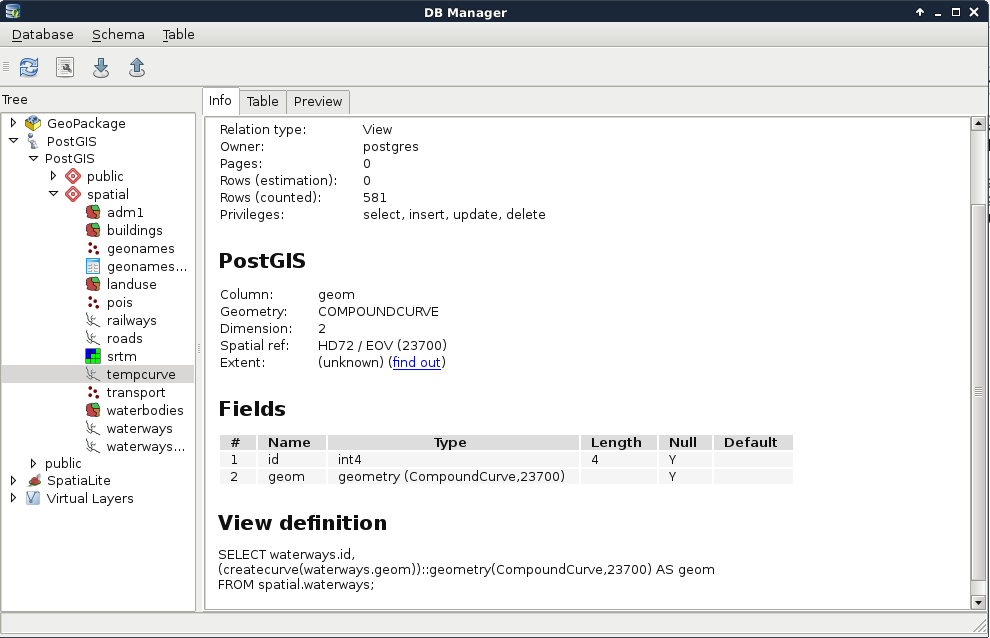
In QGIS, we can see that the new view is recognized as a view with its definition. However, if we load the layer, we also stumble on to the performance cut it introduced. As views are basically saved queries, which are executed every time the canvas is refreshed (for example, on panning and zooming), and the CreateCurve function is slow, storing this table as a view has a great performance impact:

On the other hand, those PostGIS catalogues are only queried once in a while, and it is completely affordable to sacrifice some speed to have dynamic tables without the extra hassle. On those PostGIS views, we can identify some rules for inserting, updating, and deleting rows. They are needed, as views are generally modifiable. If we try to update, insert into, or delete from a view, PostgreSQL tries to find out which tables are affected, and applies the required operations on them. To override this behavior, we can define three simple rules on views using the following scheme:

    CREATE OR REPLACE RULE tablename_event AS
     ON event TO tablename DO INSTEAD NOTHING;

We can see an example of such rules on the following screenshot:

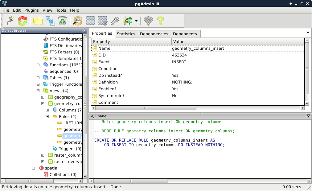
The event should be UPDATE, INSERT, or DELETE, while the tablename should be the view we would like to apply the rules on. Of course, we can do it with pgAdmin's GUI like we did before. In there, we only have to give the rule a name, select the event type, and check the Do instead checkbox. If we leave everything else blank, the simple rule given earlier gets created. By applying these rules on the three events, we can easily make our views read-only. If anyone would like to modify our tables via a protected view, those operation requests will simply bounce off the database.

What if we would like to create views with better performance? We shouldn't be so demanding, right? Well, PostgreSQL thinks otherwise, and happily offers us materialized views. These views store snapshots of the queries stored in them. We can create such a view by running the following query:

    CREATE MATERIALIZED VIEW spatial.tempcurve AS SELECT id,
     CreateCurve(geom)::geometry(CompoundCurve,23700) AS geom
     FROM spatial.waterways;

As a result, we get a view which has data in it, and is read-only by default. We cannot insert into it, update it, or remove rows from it. The only drawback is that it stores the snapshot of the query created at the time of execution. If we would like to incorporate changes in our materialized view, we have to refresh it manually as follows:

    REFRESH MATERIALIZED VIEW spatial.tempcurve;