Let's satisfy the first customer by showing the houses with correct aspect values. First of all, we need the SRTM DEM we downloaded and clipped to our study area, then transformed to our projection. If we load it, we can use GDAL's raster processing algorithms to do some terrain analysis. As QGIS does not have many tools dedicated to raster analysis, it uses external modules. This implies one very important specificity of raster analysis in QGIS--we cannot use memory layers. We have to save every intermediate result to disk. This is the case in calculating the aspect of our DEM, which you can do as follows:

1. Open Raster | Terrain Analysis | Aspect from the menu bar.
2. Select the clipped SRTM DEM as Elevation layer.
3. Specify an output, preferably in your working folder where you saved the clipped SRTM layer.
4. Click on OK:

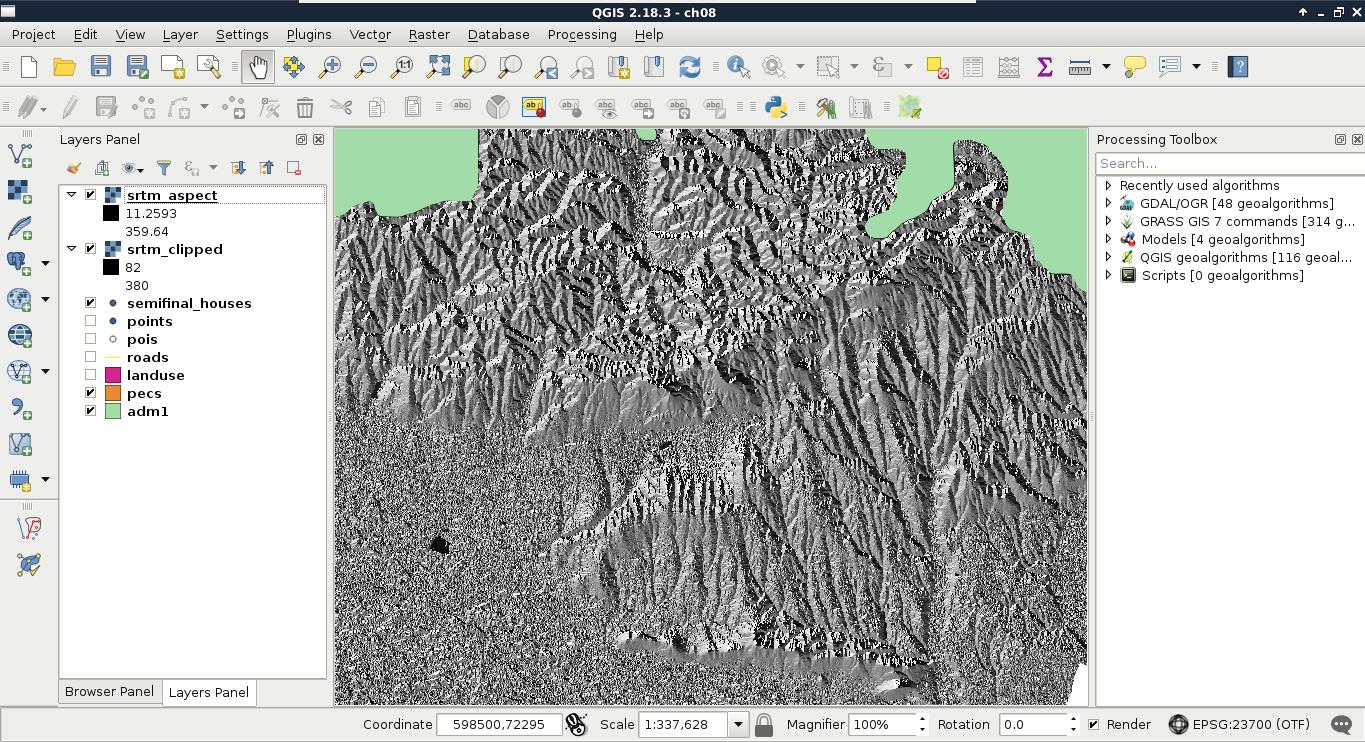
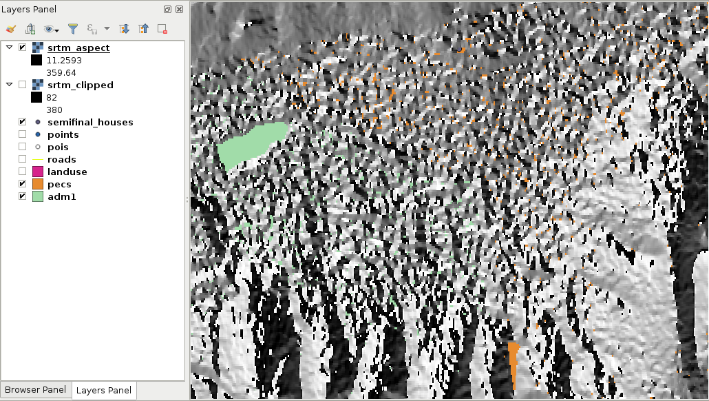
Now we have an aspect layer, which resembles the hillshading we used in a previous chapter. The only, and very significant difference is, that we did not calculate shadows cast to the surface by a light source from a specific direction, but the surface's absolute exposure. Before going on with the analysis, let's interpret the result. Values of the aspect map range from near 0 to near 360. This corresponds to exposure values expressed in degrees. More importantly, we must be able to map aspect values to directions. This sounds trivial; however, start directions can change from GIS to GIS. In QGIS, 0° and 360° correspond to North. Therefore, as we go clockwise (imagine a compass), 90° is East, 180° is South, and 270° is West. If we zoom in, and toggle the visibility of the underlying DEM, we can also see some areas without any values. There is a special value in aspect maps--flat. Flat surfaces can be denoted with a special value, such as -1, or like in our case, can be defined as NULL. We have to consider these flat values when we filter our points:

There is only one thing left--we have to sample the aspect map in the locations of our houses. Unfortunately, QGIS does not have a tool to achieve this task, but we can use GRASS GIS, which is really strong in raster analysis. Using GRASS has only one inconvenience--it won't create a column for the aspect values automatically:

1. Use Field Calculator on the filtered house layer, and add an empty field named aspect with a Decimal number (real) type. The precision value should be 3, and the expression can be a simple 0. Save the edits.
2. Open the GRASS GIS 7 commands | Vector | v.what.rast.points tool.
3. Select the houses as the vector points map.
4. Select the aspect layer as the raster map, which should be sampled.
5. Select the aspect column as the column to be updated.
6. Supply an expression which selects every feature, such as id > 0. Note that in GRASS, we do not enclose column names in quotation marks.
7. Specify an output in the Sampled field.

Now we have the houses with the sampled aspect values. Therefore, we can select the final set of houses with an expression, such as the following:

    "aspect" < 270 AND "aspect" > 90

Or, if we would like to be more restrictive, we can use this:

    "aspect" < 225 AND "aspect" > 135