Now that we have access to our layers in PostGIS, let's try some queries. Visualizing a whole layer from a database can involve a lot of traffic as databases are often on remote servers distributing all kinds of data. To have only the required data which we would like to work with, we can query those tables and visualize only the results in QGIS. As a warm up, remove the administrative boundaries layer and build an expression querying it from the database.

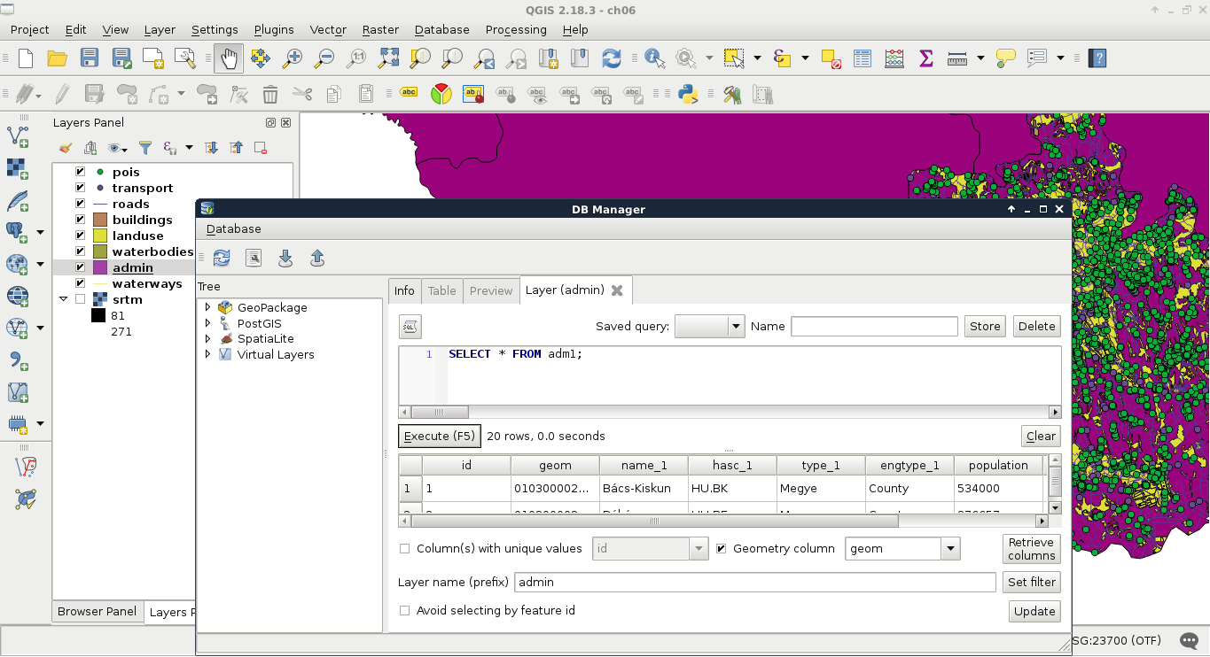
1. Open an SQL window in the database manager.
2. In Chapter 3, Using Vector Data Effectively, we discussed a traditional SQL query for selecting everything from a table. Let's use the most basic select query on our administrative boundary layer--SELECT * FROM adm1;.
3. Check the Load as new layer checkbox. We can specify the geometry column there, as it is not necessarily called geom.
4. Name the layer in the Layer name (prefix) field. Since we have access to every table in the database in the SQL builder, QGIS does not bother to find out which layers are involved in the query.
5. Click on Load now! to get the queried rows as a layer in QGIS:

One of the best things in query layers is that we can modify the query on the go. If we close the SQL window, we can reopen it with our query by right-clicking on the queried layer's item in the Layers Panel and selecting Update Sql Layer. Let's update our query and select only our study area from the table. My query will look like the following:

    SELECT * FROM adm1 WHERE name_1 = 'Baranya';

Additionally, vector data can hold a lot of attributes from which, often, only a few are relevant for our work. We can exclude some of the attribute columns by specifying only the relevant ones in the WHERE clause. There is one mandatory column that we have to include--the geometry column. Let's modify our query on the administrative boundaries layer to only have the geometry column and the corrected population density column of our study area. We don't even have to include the queried name_1 column as the rows get filtered on PostgreSQL's side.

    SELECT geom, pd_correct FROM adm1 WHERE name_1 = 'Baranya';

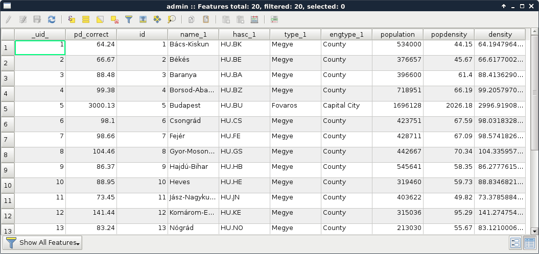
If we open the attribute table of the updated layer, we can only see two columns, _uid_ and pd_correct. We don't have to bother with the _uid_ column though, as it is QGIS's internal ID added to the attribute table of the layer.

From now on, we will recreate some of the queries we did in QGIS before. For this, we have to upload our geonames_desc.csv file to our database. Let's open it in QGIS as we did before (Add Delimited Text Layer) and import it in PostGIS like we imported our vector layers. QGIS's database manager is a convenient tool for not only loading vector layers in a PostGIS database but also for loading regular tables. We can leave every option of the import tool on their default values.

In PostGIS, we can calculate additional columns from existing ones on the fly. We can define these additional columns with their expressions as we did with regular columns and even give them a name with the alias keyword AS. Let's retrieve the whole administrative boundaries layer and, additionally, query a recalculated population density column based on the population data stored in the layer:

    SELECT *, population / (ST_Area(geom) / 1000000) AS
      density FROM adm1;

Great job! You just used your first PostGIS function, ST_Area, which returns the area of the given geometry. As we are in our local projection, we don't have to fear great distortions caused by a wrongly chosen projection. If we look at the attribute table, we can see some minor differences between the new density and the old pd_correct columns. That difference is due to the calculation of pd_correct on the surface of the WGS84 ellipsoid.

We can also do spatial queries in PostGIS. As we have features clipped to our study area, let's do something else. Select every POI inside the land use shapes. It shouldn't matter which land use shape contains the POIs, just select them all. We can do such a query with the following expression:

    SELECT p.* FROM pois p, landuse l WHERE
      ST_Intersects(p.geom, l.geom);

As we used two tables for a single query, we have to exactly define which table should be included in the results. Additionally, we can ease our work by giving a shorthand for our tables in the FROM part. We can do such a thing by adding the shorthand after the table name separated by a whitespace. Let's spice up the query a little bit. Select only those POIs which are in forest areas. If we think it through, we can achieve this by filtering the geometries of the land use layer. We can include a subquery doing just that. Modify the query as follows and click on Execute (do not load the results as the updated layer):

    SELECT p.* FROM pois p, landuse l WHERE ST_Intersects(
      p.geom, (SELECT l.geom WHERE l.fclass = 'forest'));

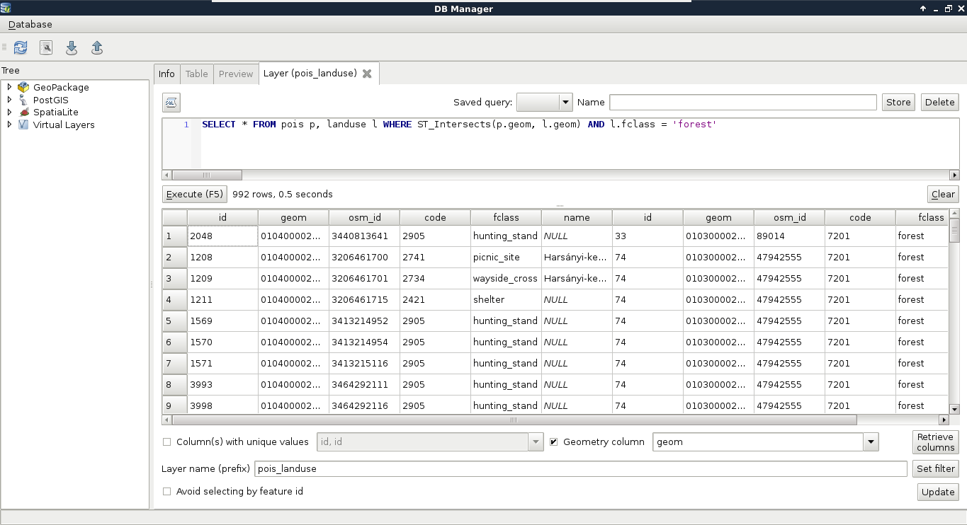
How long did it take for you? For me, it took about 80 seconds. Can you imagine QGIS loading for 80 seconds when you pan the map or zoom around? Me neither. Using subqueries in PostGIS is generally a bad way to solve problems achievable with simple queries. When we applied a filter on the land use layer and the results were correct, the filter was recalculated for every row PostGIS iterated through. PostgreSQL had no way to optimize this query and as a result it took very long. The correct way of doing this is by using a logical operator as follows:

    SELECT p.* FROM pois p, landuse l WHERE ST_Intersects(
      p.geom, l.geom) AND l.fclass = 'forest';

That's more like it. But why did it work? Because PostGIS does not make spatial queries, it creates spatial joins and applies filtering. If we alter the query to include fields from the land use table, we can see what's happening. We get every property of the intersecting land use features joined to the POIs (even their geometries). This is a classic example of an inner join:

So, there we are. Joins and spatial joins. As we saw, we can do spatial joins fairly easily-- we just have to express the spatial predict with the appropriate PostGIS function in the WHERE clause. Of course, we can also use traditional join types both in regular and spatial joins. Let's create a regular join by joining the description table to our GeoNames layer. We discussed in a previous chapter that a join in QGIS is like a left outer join in an RDBMS. Therefore, we can use LEFT OUTER JOIN in our query to create similar results.

    SELECT g.*, gd.description
      FROM geonames g
      LEFT OUTER JOIN geonames_desc gd
      ON g.featurecod = gd.code;

Let's try a spatial join as the next task. Remember when we joined our filtered GeoNames layer to our administrative boundaries layer just to have population data in our polygon layer? We can reproduce those results with the following expression:

    SELECT a.*, g.population AS g_population
      FROM adm1 a 
      INNER JOIN geonames g
      ON ST_Intersects(a.geom, g.geom) AND g.featurecod = 'ADM1';

There are two significant differences in this case. First, we only have an extract of our GeoNames layer containing points in our study area. Secondly, we already have a population column in our administrative boundaries layer. To fix the collision and make the layer readable by QGIS, we can give the population column of our GeoNames table an alias. As you can see, the inner join returned only the intersecting rows; therefore, we only got our study area back, the rest of the administrative boundaries layer got filtered out. We can get the whole layer, filled with data only where it is possible with the outer join, as stated before:

    SELECT a.*, g.population AS g_population
      FROM adm1 a 
      LEFT OUTER JOIN geonames g
      ON ST_Intersects(a.geom, g.geom) AND g.featurecod = 'ADM1';

Now  we have every feature with a g_population column filled with NULL values where there is no matching GeoNames feature. Of course, we have some other join types we can use. If our target table is in the SELECT clause and the joined table is in the JOIN clause, we can make the following joins in PostgreSQL:

• CROSS JOIN: Creates rows for every possible combination between the two tables. It is rarely usable for spatial queries. It does not need a join condition.
• INNER JOIN: Returns rows from the target table where the join condition is true. The joined table's columns are only joined there.
• LEFT OUTER JOIN: Returns every row from the target table. Where the join condition is met, the values of the joined table are included. Where not, the fields are filled with NULL values.
• RIGHT OUTER JOIN: Returns every row from the joined table. Where the join condition is met, the values of the target table are included. Where not, the fields are filled with NULL values.
• FULL OUTER JOIN: Returns every row from both the tables. There will be only completely filled rows where the join condition is true. Other rows are partially filled with NULL values. It cannot be used with spatial conditions.