The final preference was that the house should be within a 15 minutes walking distance to the train and bus stations. We could calculate the time taken to reach a point from another one on a road network using network analysis. However, that method would not respect an important factor in walking--elevation. This is a kind of nontrivial analysis done on a DEM. Although neither QGIS, nor PostGIS offer a solution for this type of analysis, GRASS GIS has just the tool for us. This tool creates a cost surface, which represents walking time in seconds from one or more input points. For this, GRASS needs a DEM and an additional friction map. With the friction map, we can fine-tune the analysis, giving weights to some of the areas. For example, we can give a very high value to buildings, making GRASS think that it's almost impossible to walk through them. The friction map must be in the raster format, therefore, our first task is to create it from our vectors. For the sake of simplicity, let's only consider buildings, forests, and parks.

1. Apply a filter on the landuse layer to only show forests and parks. The correct expression is "fclass" = 'park' OR  "fclass" = 'forest'.
2. Clip the landuse layer to the town's boundary. You can use memory layers if not stated otherwise.
3. Load the buildings layer, and clip it to the town's boundary. Save the clipped layer as a temporal layer, or to the disk.
4. Calculate the difference of the landuse layer and the buildings layer (in this order). It is convenient to not have overlapping or duplicated features in the final result. By calculating the difference of the two layers, we basically erase the buildings from the landuse layer. Save this layer as a temporal layer, or to the disk.
5. Merge the buildings and the difference layer with QGIS geoalgorithms | Vector general tools | Merge vector layers. You might want to build spatial indices on the input layers before (Properties | General | Create spatial index). Save the merged layer to the disk.

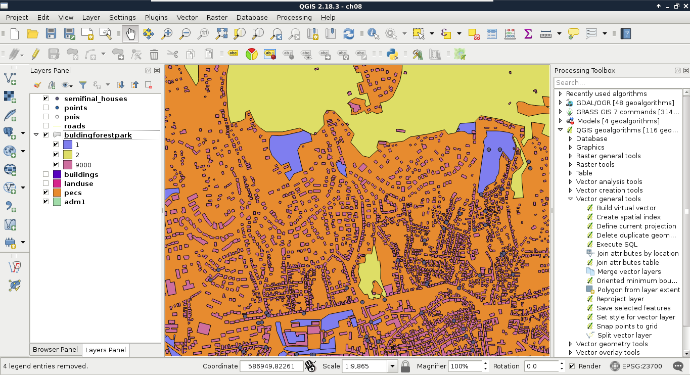
6. Give friction costs to the features using the Field Calculator. The field name should be cost, while the field type should be Whole number (integer). Friction costs represent the penalty in seconds for crossing a single meter on the surface. For buildings layer, this penalty should be an arbitrary high number, such as 9000. For parks, the penalty can be 1, while for forests, the penalty can be 2. We can assign these costs conditionally using the following expression:

        CASE
        WHEN "fclass" = 'building' THEN 9000
        WHEN "fclass" = 'forest' THEN 2
        WHEN "fclass" = 'park' THEN 1
        END

7. Save the edits and clean up (remove intermediary data):

Now we have a vector friction layer, although GRASS needs a raster layer containing penalties. To transform our vector to raster, we can use GDAL's Rasterize module from Raster | Conversion. This module can create rasters from input vectors, although we should keep the differences of the two data models in mind:

• Rasters usually hold a single attribute, while vectors hold many. We have to choose a single attribute to work with.
• Rasters have a fixed resolution, while the concept of resolution does not apply to vector data, at least in this literal sense. We will lose data, and we have to choose how much we would like to lose. By choosing a very low spatial resolution, we can make our calculations very slow, while, if we choose too high value, we can get a faulty result (Appendix 1.10).
• As rasters consist of coincident cells, there is no guarantee the vector layer's bounds will match the resulting raster layer's bounds. Furthermore, if we use raster (matrix) algebra, there is no guarantee that the rasterized layer will fully overlap with other inputs. GRASS and GDAL handle these cases really well, although this is not universally true for every GIS.

Now that we have a concept about vector to raster transformation, let's create our friction map as follows:

1. Open the Raster | Conversion | Rasterize tool from the menu bar.
2. Choose the friction vector layer as an input, and the cost column as Attribute field.
3. Browse an output. Ignore the warning about creating a new raster. GDAL will handle that just right.
4. Choose the Raster resolution in map units per pixel radio box.
5. Provide 2 (or the equivalent if you use a unit other than meters) in both the Horizontal and Vertical fields.

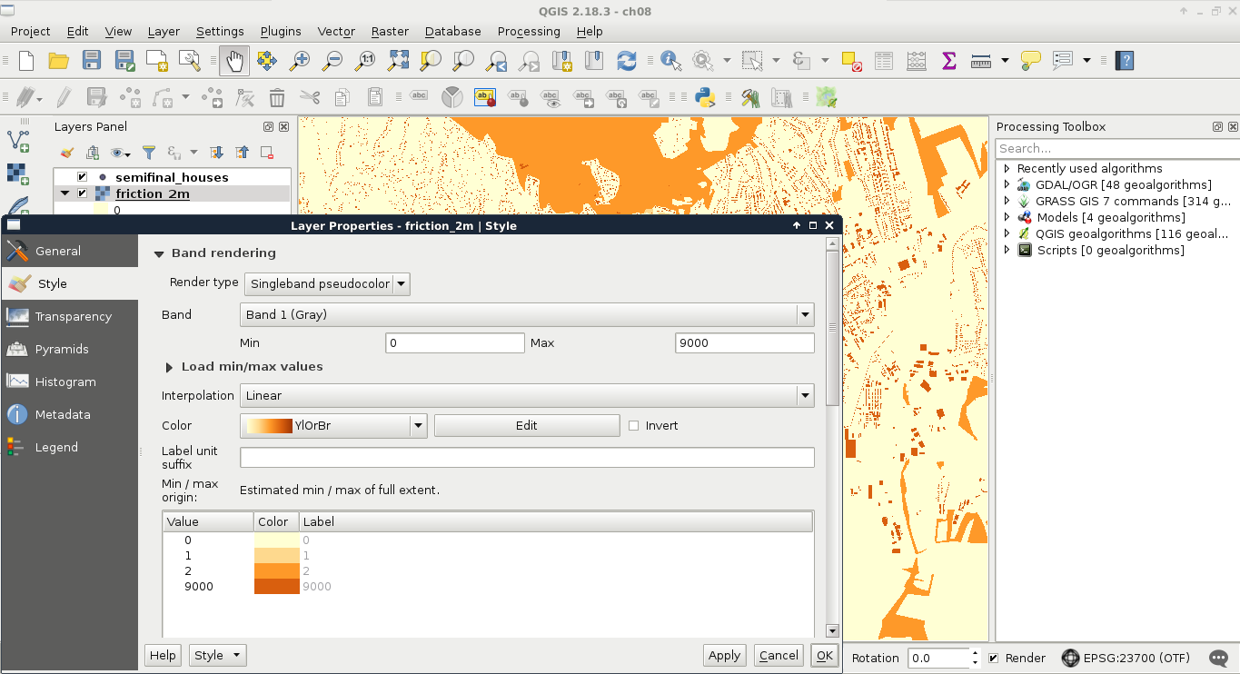
6. The result is most likely a sole black raster. If you would like to see the different values, use a single band styling mode (Properties | Style), then specify the 0, 1, 2, and 9000 values as intervals:

7. As the new raster map has most likely a custom projection with the same parameters as our local projection, assign the local projection to it instead. Otherwise, GRASS will complain about the projection mismatch. We can select our local projection in Properties | General | Coordinate reference system:

Besides the friction map, GRASS also needs an elevation map. However, we have some work to do on our SRTM DEM. First, as we have two raster layers with two resolutions, and it is no trivial matter for GRASS which one to choose, we have to resample our DEM to 2 meters. We should also clip the elevation raster to our town's boundary in order to reduce the required amount of calculations.

1. Open the SRTM DEM transformed to our local projection.
2. Select the Raster | Extraction | Clipper tool.
3. Select the DEM as the input layer, and browse an output layer.
4. Check the No data value box, thus, rasters outside of the town's boundary get NULL values.
5. Choose the Mask layer radio button.
6. Specify the town's boundary as a mask layer.

7. Check the Crop the extent of the target dataset to the extent of the cutline box, and run the tool.
8. Open the Raster | Align Rasters tool.
9. With the plus icon, add the clipped DEM to the raster list, and specify an output.
10. Check the Cell Size box, and provide the same cell size that the friction layer uses.
11. Run the tool.

The final parameter we should provide is a vector layer with a number of points representing starting points. We need two cost layers, one for the bus stations, and one for the railway stations. These data can be accessed from the transport OSM layer we inserted into PostGIS. Let's load that layer, and clip it to the town's boundary. We can store the result in a memory layer. Now we are only a few steps away from the cost surfaces:

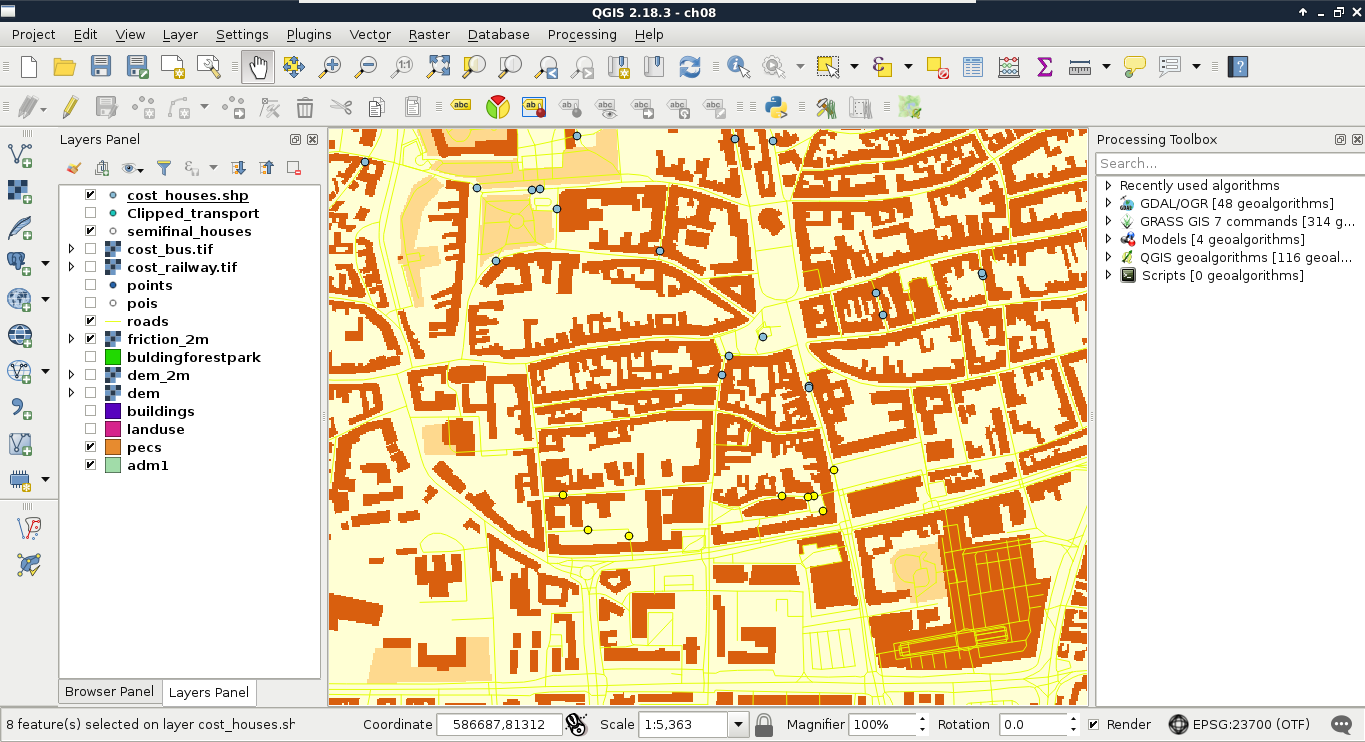
1. Filter the clipped transport layer to only show railway stations first with the expression "fclass" = 'railway_station'.
2. Examine the railway stations. Are there any local stations which are irrelevant for our analysis? If there are, delete those points. Start an edit session with Toggle Editing, select the Select Features by area or single click tool, select an irrelevant station, then click on the Delete Selected button. After every local station is removed, save the edits and exit the edit session.
3. Are there any stations inside buildings? If there are, move them out, as they will produce incorrect results. Start an edit session, select the Move feature(s) tool, and move the problematic points outside of the buildings. Finally, save the edits, and exit the edit session.
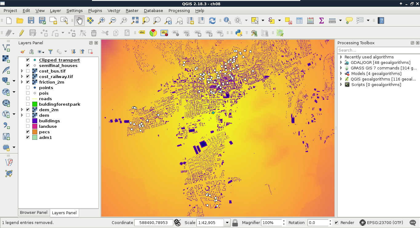
4. Create the cost surface with the GRASS GIS 7 commands | Raster | r.walk.points tool. The input elevation map should be the SRTM layer clipped to the town's boundary, the input raster layer containing friction costs is our rasterized friction layer, and the start points is the filtered, edited transport layer. All other parameters can be left with their default values.

If we style the result, we can see how much time it takes to reach our houses from the railway stations. Now we have to repeat the previous steps with bus stations. To filter bus stations, we can use the expression "fclass" = 'bus_station':

Almost there. We are only one step away from the final result--we need to sample both the cost maps at the houses' locations. Let's do this by following the steps we took earlier in this chapter:

1. Create two new fields for the houses layer with the names railway and bus using the Field Calculator. The precision and the type do not really matter in this case, as the costs are in seconds. They must have a numeric type though. The expression can be a single 0. Don't forget to save the edits, and exit the edit session once you have finished.
2. Use the GRASS GIS 7 commands | Vector | v.what.rast.points tool for sampling the first raster layer. Use a general expression, like id > 0, and save the result as a temporary layer.
3. Set the CRS of the output layer to the currently used projection in Properties | General | Coordinate reference system. GRASS applied its own definition of the same projection to the output, and will complain if it thinks that the projections of the input layers do not match.

4. Use the same tool again to sample the second raster. The input layer this time must be the output of the previous step. Save this result to the working folder.
5. Select preferred locations from the output with an expression. As the values are in seconds, we can build the expression "railway" / 60 <= 15 AND "bus" / 60 <= 15 to select the relevant houses. If there are no matches, try to use a logical OR between the two queries: