What we have now are three layers containing raw distance data. As these data are part of different criteria, we cannot directly compare them; we need to make them comparable first. We can do this by normalizing our data, which is also called fuzzification. Fuzzy values (μ) are unitless measures between 0 and 1, showing some kind of preference. In our case, they show suitability of the cells for a single criterion. As we discussed earlier, 0 means 0% (not suitable), while 1 means 100% (completely suitable).

The problem is that we need to model how values between the two edge cases compare to the normalized fuzzy values. For this, we can use a fuzzy membership function, which describes the relationship between raw data (crisp values) and fuzzy values. There are many membership functions with different parameters. The most simple one is the linear function, where we simply transform our data to a new range. This transformation only needs two parameters--a minimum and a maximum value. Using these values, we can  transform our data to the range between 0 and 1. Of course, a linear function does not always fit a given phenomenon. In those cases, we can choose from other functions, among which the most popular in GIS are the sigmoid and the J-shaped functions:

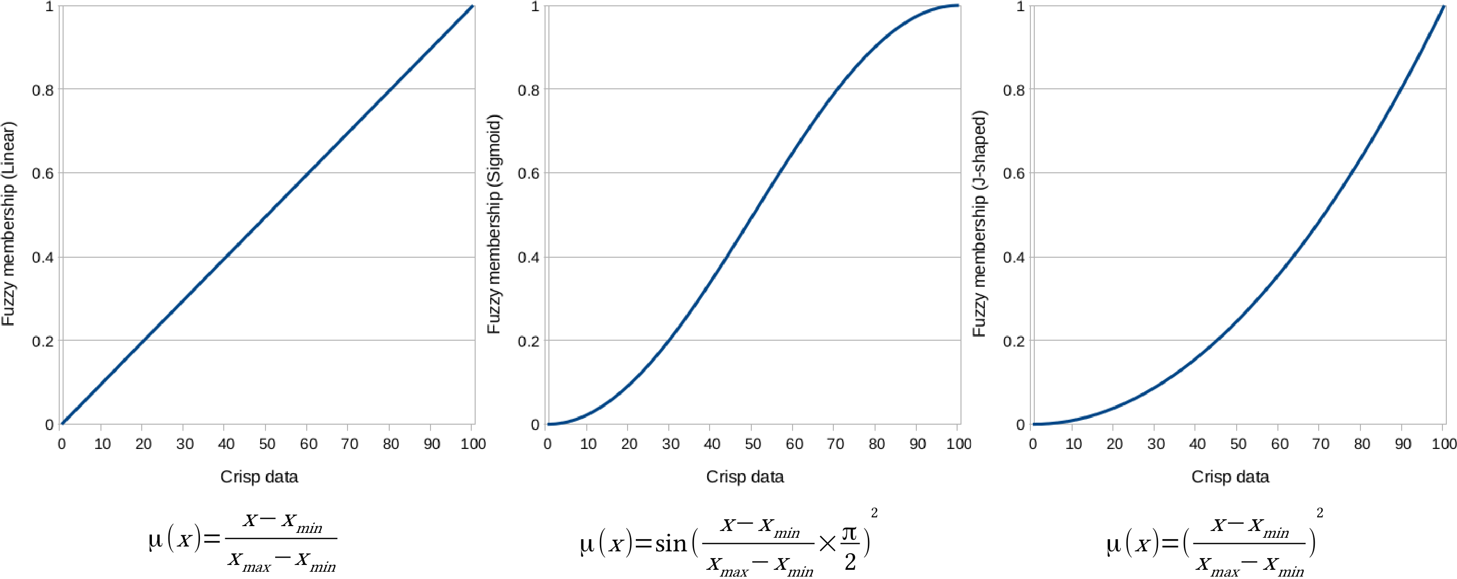
To solve this problem, we have to interpret the membership functions, and choose the appropriate one for our crisp data. The various membership functions are explained as follows:

• Linear: The simplest function, which assumes a direct, linear relationship between crisp and fuzzy values. It is good for the roads layer with the minimum value of 0 and the maximum value of 5000. We have to handle distances over 5000 meters manually, and invert the function, as cells closer to the roads are more suitable.
• Sigmoid: This function starts slowly, then increases steeply, and then ends slowly. It is good for the mean coordinates map, as the benefit of being near to the settlements' center of mass diminishes quickly on the scale of the whole study area. We have to use the minimum value of 0, and the maximum value of the layer. Additionally, we have to invert the function for this layer, too.
• J-shaped: A quadratic function which starts slowly, and then increases rapidly. It can be used with the waters layer, as it is safer to assume a quadratic relationship on a risk factor, when we do not have information about the actual trends. We can use the minimum value of 200 and the maximum value of the layer.

First, let's use the J-shaped membership function on the waters layer, as follows:

1. We have a minimum value of 200 meters at hand, however, we need to find out the maximum value. To do this, go to Properties | Metadata. The STATISTICS_MAXIMUM entry holds the maximum value of the layer. Round it up to the nearest integer, and note down that number.
2. Open a raster calculator, and create an expression from the J-shaped function, the minimum, and the maximum values. Handle values less than the minimum value in a conditional manner. Save the result as a GeoTIFF file. The final expression should be similar to the following:

        ("waters_dist@1" <= 200) * 0 + ("waters_dist@1" > 200) *
         (("waters_dist@1" - 200) / (max - 200)) ^ 2

Next, we should apply the linear membership function to the roads layer as follows:

1. Open a raster calculator, and create an expression from the inverted linear function, the minimum value of 0, and the maximum value of 5000. Handle values more than 5000 meters in a conditional manner. Save the result as a GeoTIFF file. The final expression should be similar to the following:

        ("roads_dist@1" > 5000) * 0 + ("roads_dist@1" <= 5000) *
         (1 - ("roads_dist@1" / 5000))

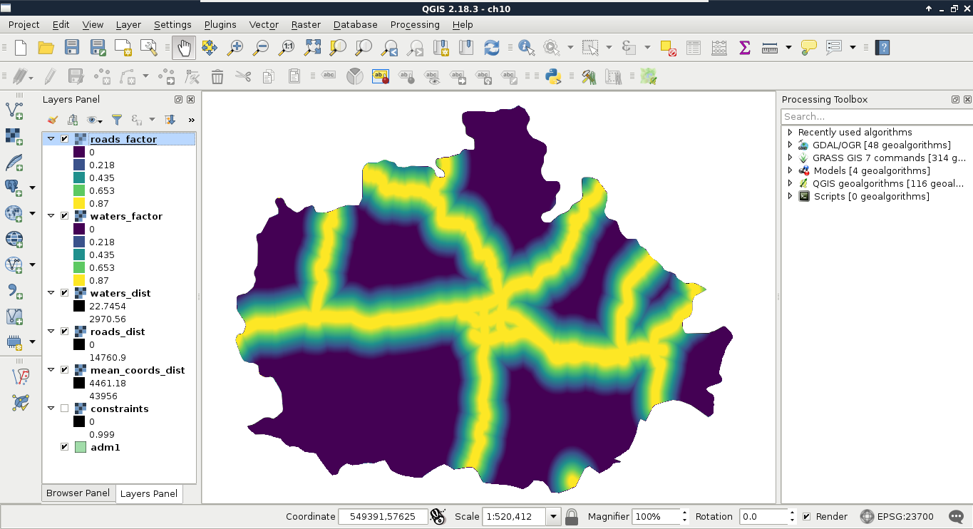
By running the expression, we should be able to see two of our factor layers:

Finally, we use the sigmoid function for the mean coordinates layer like this:

2. We know the minimum value is 0, however, we need to find out the maximum value. Check it in Properties | Metadata, round it up to the nearest integer, and note down the value.
3. Open a raster calculator, and create an expression from the minimum and maximum values, and from the inverted sigmoid function. We do not have access to π, although we can hard code it as 3.14159. Save the result as a GeoTIFF file:

        1 - sin("mean_coords_dist@1" / max * (3.14159 / 2)) ^ 2