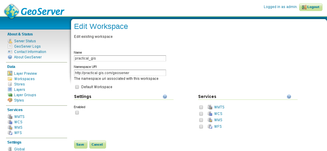
Before adding some data to GeoServer, let's create a new workspace for it. This way, the data will be safely separated, and we will be able to access the content by using a virtual endpoint:

1. Open Data | Workspaces.
2. Select Add new workspace.
3. Specify a name for the workspace in the Name field.
4. Give a namespace for the workspace in the Namespace URI field. The namespace must be a URI (that is, a URL or a URN). It does not have to point to an existing resource, only its uniqueness is what matters (compared to the URIs of the other workspaces). For example, a URL can be http://practical-gis.com/geoserver, while a URN can be urn:practical-gis:geoserver:

Now we can start defining stores for our data sources. GeoServer does not create internal copies of the input data. It only uses references to the input files or databases, and reads the underlying spatial data on demand:

1. Go to Data | Stores and select Add new Store.

Although GeoServer has somewhat limited knowledge about spatial formats, it still offers stores for the three formats we used previously in this book--Shapefile, PostGIS, and GeoTIFF.

2. Select PostGIS.
3. Set the Workspace to the one we created previously.
4. Give a name to the data source. The name won't be used by the services, although it must be a unique one.
5. Provide the name of the database in the database field. If you followed the book's naming conventions, it is spatial.
6. Provide the name of the schema containing spatial tables in the schema field.

7. Provide the username, and optionally, the password. Although it should be safe to use a PostgreSQL role with write privilege, it is a good practice to use double protection if we do not intend to write PostGIS tables from GeoServer. Therefore, we should use the public role we created with the corresponding password. If you are on a Unix system, the password field can be left blank:

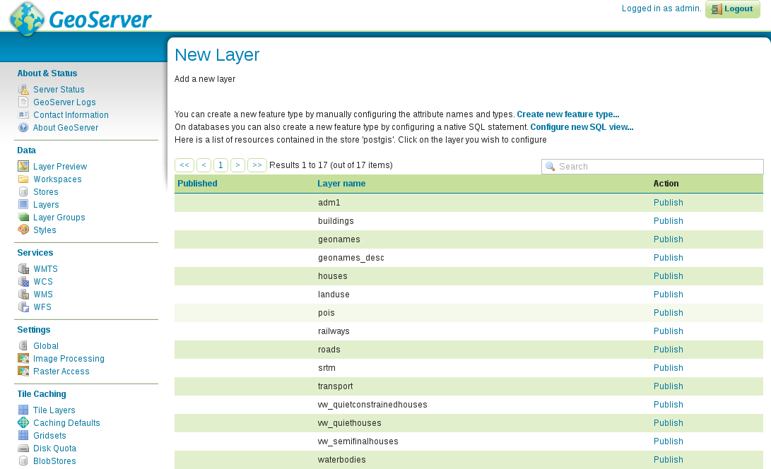
As you can see, if we use a store which can provide multiple layers, we can access every layer by their names. On the other hand, if the store is a single file which can contain only one layer, we can only access that single layer from the specific store. Before publishing a layer, let's add three more single file stores.

8. Open Add new Store from Data | Stores again.
9. Select the Shapefile option.
10. Select the workspace we created for our data.
11. Give a name to the store.
12. Browse out the shapefile containing suitable areas from our MCE analysis in the Shapefile location field by clicking on Browse.
13. Select the appropriate character encoding. Probably, it is UTF-8.
14. Save the store with the Save button, and return to the Add new Store page.
15. Select the GeoTIFF format, and choose the correct workspace.
16. Give this raster store a name, and browse out the suitability layer from the results of the MCE analysis.
17. Save the store with the Save button.
18. Add the clipped SRTM layer in the local projection we used with QGIS the same way as the suitability layer.

As we now have our data sources configured, we can start publishing relevant layers. Let's start with some of our vector layers:

1. Open Data | Layers.
2. Select Add a new layer.
3. Select one of our newly defined stores (for example, suitable areas).
4. Find a layer to publish, and click on its Publish option.
5. Supply a name for the layer if the default one is not appropriate.
6. Look at the Coordinate Reference Systems section. GeoServer will try its best to find out the CRS of the layer in the Native SRS field. If it can successfully find the corresponding SRID, it automatically fills out the Declared SRS field (that is, the default CRS of the published layer). If it cannot, we should know the EPSG code of the layer's CRS. In this case, we have to provide it in the Declared SRS field, and leave the Force declared option selected. This way, GeoServer will not care about the original CRS of the layer; it will apply the one we provided on it.
7. Calculate the bounds of the layer automatically by clicking on the Compute from data option in the Bounding Boxes section.
8. Calculate the WGS84 bounds of the layer by clicking on the Compute from native bounds option.
9. Publish the layer by clicking on the Save button.
10. Repeat the steps for the other required vector layers. We will need the administrative boundaries, the GeoNames layer, the land use, the roads, the waterways, and the water bodies.

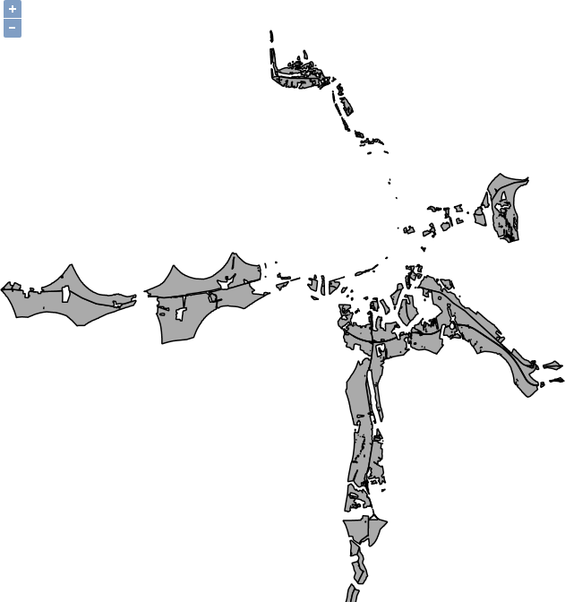
Now we have a published layer, which we can preview easily from GeoServer. The only thing we have to do is to go to Data | Layer Preview, and select the OpenLayers option in the row of the newly published layer. The result shows what the layer will look like when accessed through GeoServer's WMS service. Although GeoServer uses OpenLayers for creating its previews, the map's content will look the same in any other web-mapping application.

The suitable areas layer in the preview window should look like the following:

It's time to publish some raster layers. Publishing raster layers is a little different, but only requires one extra consideration:

1. Open Data | Layers, add a new layer, and select the suitability layer from its store.
2. The bounding box is automatically calculated this time, however, the default option for reprojecting is Reproject native to declared. It is completely useless when the native and declared SRSs are the same, while it is harmful if GeoServer cannot identify the CRS of the raster data correctly. Set it to Force declared.
3. Repeat the steps for the SRTM raster.

Now we can require individual layers, but how can we create compositions? Well, of course, we can define multiple layer names in a single GetMap request, although this approach can be quite inconvenient, especially, when we would like to stack a lot of layers. On the other hand, GeoServer has the capability of grouping layers to form a server-side composition. The only limitation of this approach is that it can only be used for WMS requests with layers in a single workspace:

1. Open Data | Layer Groups.
2. Select the Add new layer group option.
3. Name the layer group, give a descriptive title, and select the workspace we are working with.
4. Supply the EPSG code of our local projection in the Coordinate Reference System field (for example, EPSG:23700).
5. One by one, add every layer from the road map composition we made in QGIS earlier using Add Layer.
6. Click on Generate Bounds to compute the bounding box of the composition automatically.
7. Define the correct layer order by using the green arrows in the layer list. The list defines the drawing order, therefore, the first item is drawn at the bottom, while the last layer will be at the top.
8. Save the composition with the Save button.

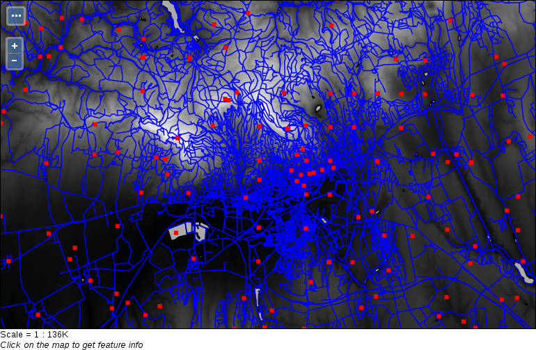
If we preview the newly created layer group, we can see the raw composition, that is, every component with their default styling stacked on each other. Now it is only a matter of styling to get a similar map like in our QGIS project: