The next flaw we correct is much less obvious and could be argued to be an error. The background of our data frame is exactly the same as the rest of the paper. This can introduce some ambiguity, which we can resolve by changing the background in our study area to another color and creating an additional Other category for land use in our legend. The easiest way to do this would be adding a fill to the administrative boundary and pulling it down to the bottom of the layer list, therefore the rendering pipeline. The problem with this approach is our srtm layer gets blended into these new areas, creating a lot of noise. Fortunately, with some clever processing, we can create the negative of our land use layer using the following steps:

1. Select QGIS geoalgorithms | Vector overlay tools | Difference from the Processing Toolbox.
2. Supply the filtered administrative boundary as Input layer, and the land use layer as Difference layer. Save the result to a memory layer.
3. Pull the result just above the srtm layer, and style it using a very light color with no outline.
4. In the new layer's Style tab, select the Fill parent category. Next to Color, select the interactive color chooser with the down arrow next to the field. Click on Copy color.
5. Open the land use layer's Style tab, add a new category with the plus button.
6. Set the Label to Other, the Filter to FALSE, and paste the copied color using the interactive color chooser of its Fill parent style category. Finally, remove the outline from the style:

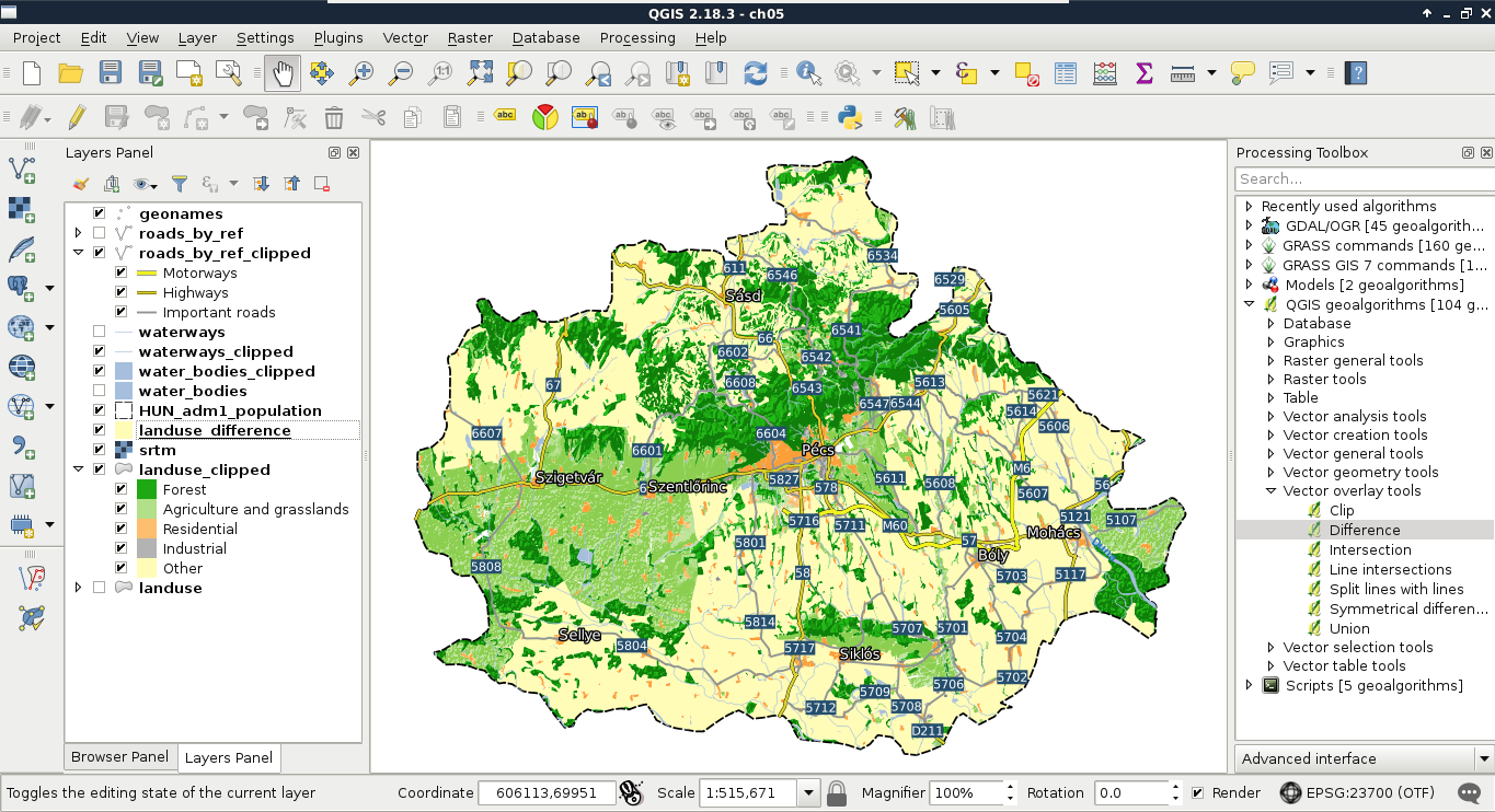
The Difference tool returns the difference between the geometries of the first layer and the second layer. It basically erases the second layer from the first layer and returns the results. Some of QGIS's geoalgorithms are error-prone and even can cause a crash. For example, the Difference tool crashed for me. If this happens, we can always choose GRASS GIS's equivalent algorithm. GRASS GIS is a professional, very stable, and quite fast software, although it has a quite steep learning curve and assumes its users are proficient GIS users with some programming knowledge.

We will discuss the peculiarities of GRASS GIS in a later chapter. For now, the required tool for achieving the same result is v.overlay, which can be accessed from GRASS (GIS 7) commands | Vector in the Processing Toolbox. This tool is a great example of GRASS GIS's philosophy. It requires two input layers (A and B), and we must be able to distinguish between them. The A layer is the input layer, while the B layer is the reference, or mask layer. Therefore, we need to specify our administrative boundaries layer for A and our land use layer for B. This tool groups some of the mostly identical basic geoalgorithms. The specified operator decides which algorithm it should run. The AND means clip, the OR means union, the NOT means difference, while the XOR means symmetrical difference (Appendix 1.3). After we define not as the operator, we only have to choose an output type, which cannot be a memory layer for any GRASS algorithm. We can either save the result to a temporary file or specify an output. As the two approaches are almost the same (disk usage occurs in both cases), specifying the output is recommended as we can restore it later from the saved project.