Table of Contents for
Practical GIS

Version ebook / Retour

Cover image for bash Cookbook, 2nd Edition Practical GIS by Gábor Farkas Published by Packt Publishing, 2017
  1. Practical GIS
  2. Title Page
  3. Copyright
  4. Credits
  5. About the Author
  6. About the Reviewer
  7. www.PacktPub.com
  8. Customer Feedback
  9. Dedication
  10. Table of Contents
  11. Preface
  12. What this book covers
  13. What you need for this book
  14. Who this book is for
  15. Conventions
  16. Reader feedback
  17. Customer support
  18. Downloading the example code
  19. Downloading the color images of this book
  20. Errata
  21. Piracy
  22. Questions
  23. Setting Up Your Environment
  24. Understanding GIS
  25. Setting up the tools
  26. Installing on Linux
  27. Installing on Windows
  28. Installing on macOS
  29. Getting familiar with the software
  30. About the software licenses
  31. Collecting some data
  32. Getting basic data
  33. Licenses
  34. Accessing satellite data
  35. Active remote sensing
  36. Passive remote sensing
  37. Licenses
  38. Using OpenStreetMap
  39. OpenStreetMap license
  40. Summary
  41. Accessing GIS Data With QGIS
  42. Accessing raster data
  43. Raster data model
  44. Rasters are boring
  45. Accessing vector data
  46. Vector data model
  47. Vector topology - the right way
  48. Opening tabular layers
  49. Understanding map scales
  50. Summary
  51. Using Vector Data Effectively
  52. Using the attribute table
  53. SQL in GIS
  54. Selecting features in QGIS
  55. Preparing our data
  56. Writing basic queries
  57. Filtering layers
  58. Spatial querying
  59. Writing advanced queries
  60. Modifying the attribute table
  61. Removing columns
  62. Joining tables
  63. Spatial joins
  64. Adding attribute data
  65. Understanding data providers
  66. Summary
  67. Creating Digital Maps
  68. Styling our data
  69. Styling raster data
  70. Styling vector data
  71. Mapping with categories
  72. Graduated mapping
  73. Understanding projections
  74. Plate Carrée - a simple example
  75. Going local with NAD83 / Conus Albers
  76. Choosing the right projection
  77. Preparing a map
  78. Rule-based styling
  79. Adding labels
  80. Creating additional thematics
  81. Creating a map
  82. Adding cartographic elements
  83. Summary
  84. Exporting Your Data
  85. Creating a printable map
  86. Clipping features
  87. Creating a background
  88. Removing dangling segments
  89. Exporting the map
  90. A good way for post-processing - SVG
  91. Sharing raw data
  92. Vector data exchange formats
  93. Shapefile
  94. WKT and WKB
  95. Markup languages
  96. GeoJSON
  97. Raster data exchange formats
  98. GeoTIFF
  99. Clipping rasters
  100. Other raster formats
  101. Summary
  102. Feeding a PostGIS Database
  103. A brief overview of databases
  104. Relational databases
  105. NoSQL databases
  106. Spatial databases
  107. Importing layers into PostGIS
  108. Importing vector data
  109. Spatial indexing
  110. Importing raster data
  111. Visualizing PostGIS layers in QGIS
  112. Basic PostGIS queries
  113. Summary
  114. A PostGIS Overview
  115. Customizing the database
  116. Securing our database
  117. Constraining tables
  118. Saving queries
  119. Optimizing queries
  120. Backing up our data
  121. Creating static backups
  122. Continuous archiving
  123. Summary
  124. Spatial Analysis in QGIS
  125. Preparing the workspace
  126. Laying down the rules
  127. Vector analysis
  128. Proximity analysis
  129. Understanding the overlay tools
  130. Towards some neighborhood analysis
  131. Building your models
  132. Using digital elevation models
  133. Filtering based on aspect
  134. Calculating walking times
  135. Summary
  136. Spatial Analysis on Steroids - Using PostGIS
  137. Delimiting quiet houses
  138. Proximity analysis in PostGIS
  139. Precision problems of buffering
  140. Querying distances effectively
  141. Saving the results
  142. Matching the rest of the criteria
  143. Counting nearby points
  144. Querying rasters
  145. Summary
  146. A Typical GIS Problem
  147. Outlining the problem
  148. Raster analysis
  149. Multi-criteria evaluation
  150. Creating the constraint mask
  151. Using fuzzy techniques in GIS
  152. Proximity analysis with rasters
  153. Fuzzifying crisp data
  154. Aggregating the results
  155. Calculating statistics
  156. Vectorizing suitable areas
  157. Using zonal statistics
  158. Accessing vector statistics
  159. Creating an atlas
  160. Summary
  161. Showcasing Your Data
  162. Spatial data on the web
  163. Understanding the basics of the web
  164. Spatial servers
  165. Using QGIS for publishing
  166. Using GeoServer
  167. General configuration
  168. GeoServer architecture
  169. Adding spatial data
  170. Tiling your maps
  171. Summary
  172. Styling Your Data in GeoServer
  173. Managing styles
  174. Writing SLD styles
  175. Styling vector layers
  176. Styling waters
  177. Styling polygons
  178. Creating labels
  179. Styling raster layers
  180. Using CSS in GeoServer
  181. Styling layers with CSS
  182. Creating complex styles
  183. Styling raster layers
  184. Summary
  185. Creating a Web Map
  186. Understanding the client side of the Web
  187. Creating a web page
  188. Writing HTML code
  189. Styling the elements
  190. Scripting your web page
  191. Creating web maps with Leaflet
  192. Creating a simple map
  193. Compositing layers
  194. Working with Leaflet plugins
  195. Loading raw vector data
  196. Styling vectors in Leaflet
  197. Annotating attributes with popups
  198. Using other projections
  199. Summary
  200. Appendix

Proximity analysis in PostGIS

The first task in Chapter 8, Spatial Analysis in QGIS was to select every house which is at least 200 meters away from busy roads and 500 meters away from industrial areas. To complete this task, we created buffer zones around the problematic features and areas, calculated their union, and selected every disjoint house. Following the same approach, we can use two functions of PostGIS--ST_Intersects and ST_Buffer. We do not have to discuss ST_Intersects again, as we have already used it several times. ST_Buffer, on the other hand, is a different function. It does not act as a filtering function, but it creates and returns new geometries based on the input geometries and buffer distances. To buffer the busy roads of our roads layer, we can create the following expression:

    SELECT ST_Buffer(geom, 200) AS geom
FROM spatial.roads r
WHERE r.fclass LIKE 'motorway%' OR r.fclass LIKE 'primary%';

If we execute the expression with the Execute button, we can see the resulting geometries, while, if we load the result as a layer by checking the Load as a new layer box, filling out the required fields, and selecting Load now!, we can see the buffered roads in QGIS:

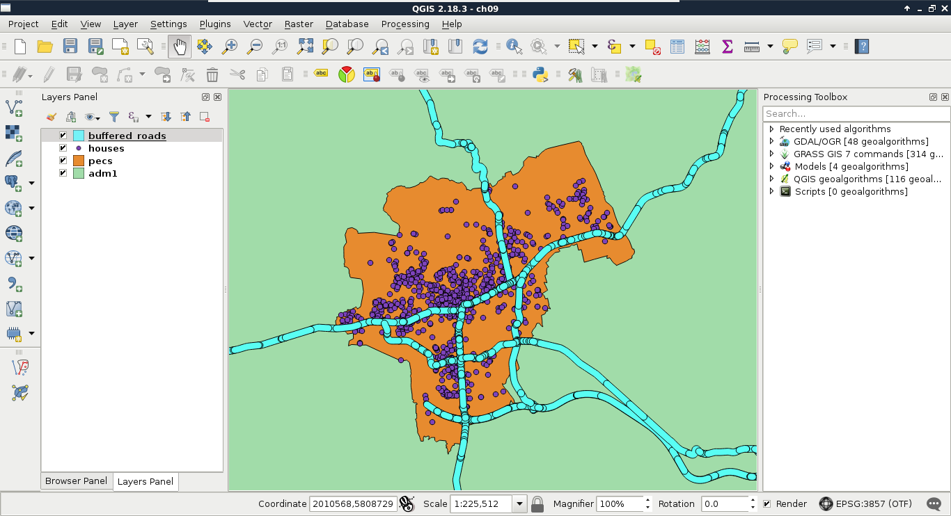
It is as easy as that. PostGIS iterates through the filtered roads, and buffers them on a row-by-row basis. It does not dissolve the results, or do anything else, but just returns the raw buffered geometries, and additionally, the attributes if we ask for them. As we will only use the geometries of the roads, we do not need any other attributes.

As PostGIS executes spatial functions on a row-by-row basis, we can create variable-sized buffer zones by specifying a numeric attribute field instead of the constant number as the second argument of ST_Buffer.

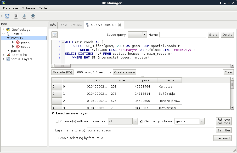
The only thing left to do is to check if our houses intersect with the buffer zones. As we only need a subset of the roads, which is effectively a subquery, we should precalculate the buffer zones in a CTE (Common Table Expression) table by using the WITH keyword as follows:

    WITH main_roads AS (
SELECT ST_Buffer(geom, 200) AS geom
FROM spatial.roads r
WHERE r.fclass LIKE 'primary%' OR r.fclass LIKE 'motorway%')
SELECT h.* FROM spatial.houses h, main_roads mr
WHERE NOT ST_Intersects(h.geom, mr.geom);

Make sure to only execute the query; do not load as a layer. What did you get as a result? For me, this query returned more than 1 million rows. That's definitely a cross join between the individual buffer zones and the houses. Let's see if the results are correct, though. We can select only unique rows by using the DISTINCT operator after the SELECT keyword:

    WITH main_roads AS (
SELECT ST_Buffer(geom, 200) AS geom FROM spatial.roads r
WHERE r.fclass LIKE 'primary%' OR r.fclass LIKE 'motorway%')
SELECT DISTINCT h.* FROM spatial.houses h, main_roads mr
WHERE NOT ST_Intersects(h.geom, mr.geom);

The preceding query returns 1000 rows. That's the number of features we have in our houses layer.

By creating a cross join, PostgreSQL returned every occurrence, where a house is disjoint with a buffer zone. That is, it returned every house multiple times. The magic we can use to solve this problem is to calculate the union of the buffer zones with ST_Union:

    WITH main_roads AS (
SELECT ST_Union(ST_Buffer(geom, 200)) AS geom
FROM spatial.roads r
WHERE r.fclass LIKE 'primary%' OR r.fclass LIKE 'motorway%')
SELECT h.* FROM spatial.houses h, main_roads mr
WHERE NOT ST_Intersects(h.geom, mr.geom);

You must be wondering if this even makes any sense. If PostGIS goes row by row, why would it matter if we use union on every individual buffered geometry? The answer is that ST_Union is an aggregate function. Aggregate functions in PostGIS behave differently when they are called with one argument in a SELECT clause. They act on every returned row, and return a single geometry if there are no additional groupings defined. Now that the main_roads table has a single row, PostgreSQL behaves nicely, and returns only the disjoint features in less than a second.

The only thing left to do is to query houses which do not reside in the 500 meters buffer zone of industrial areas. For this, we need an additional CTE table with the union of the buffered industrial areas. In PostgreSQL, we can create multiple virtual tables in a single WITH clause by separating them with commas as follows:

    WITH main_roads AS (
SELECT ST_Union(ST_Buffer(geom, 200)) AS geom
FROM spatial.roads r
WHERE r.fclass LIKE 'primary%' OR r.fclass LIKE 'motorway%'),
industrial_areas AS (
SELECT ST_Union(ST_Buffer(geom, 500)) AS geom
FROM spatial.landuse l
WHERE l.fclass = 'industrial' OR l.fclass = 'quarry')
SELECT h.* FROM spatial.houses h, main_roads mr,
industrial_areas ia
WHERE NOT ST_Intersects(h.geom, mr.geom) AND NOT
ST_Intersects(h.geom, ia.geom);

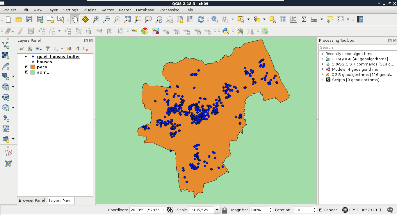
Quite a complex query, isn't it? On the other hand, it still returns the correct houses in less than a second, which is a serious performance boost. Let's load the results as a layer in QGIS, named something like quiet_houses_buffer:

What is really great about PostGIS is that we do not have to rely on traditional ways of analysis. We can cook up new methods if they can be done on a row-by-row basis, and return correct results. For example, we do not have to buffer the constraint features, just measure their distances to the houses with ST_Distance. This way, we can use a more lightweight aggregate function--ST_Collect. It does not calculate the union of the input geometries, but just merges them into a single one. If we supply polygons, the resulting geometry will be a multipart polygon containing the input polygons as members.

Using ST_Collect with ST_Intersects does not work out well every time. It is more reliable to use ST_Union with ST_Intersects.

Let's create a query using ST_Distance and ST_Collect:

    WITH main_roads AS (
SELECT ST_Collect(geom) AS geom
FROM spatial.roads r
WHERE r.fclass LIKE 'primary%' OR r.fclass LIKE 'motorway%'),
industrial_areas AS (
SELECT ST_Collect(geom) AS geom FROM spatial.landuse l
WHERE l.fclass = 'industrial' OR l.fclass = 'quarry')
SELECT h.* FROM spatial.houses h, main_roads mr,
industrial_areas ia
WHERE ST_Distance(h.geom, mr.geom) > 200 AND ST_Distance(
h.geom, ia.geom) > 500;

This method has a similar performance to the last one; however, it returned fewer features for me. If you experienced the same, load the results of this query in QGIS, and examine the difference.