Road data from OpenStreetMap comes with a classification, which is very useful for creating road maps. This classification is stored in the fclass column in our layer. If we create a categorized symbology based on that column, we can see that there are a lot of classes. From those classes, only a few are appropriate to show at this scale:

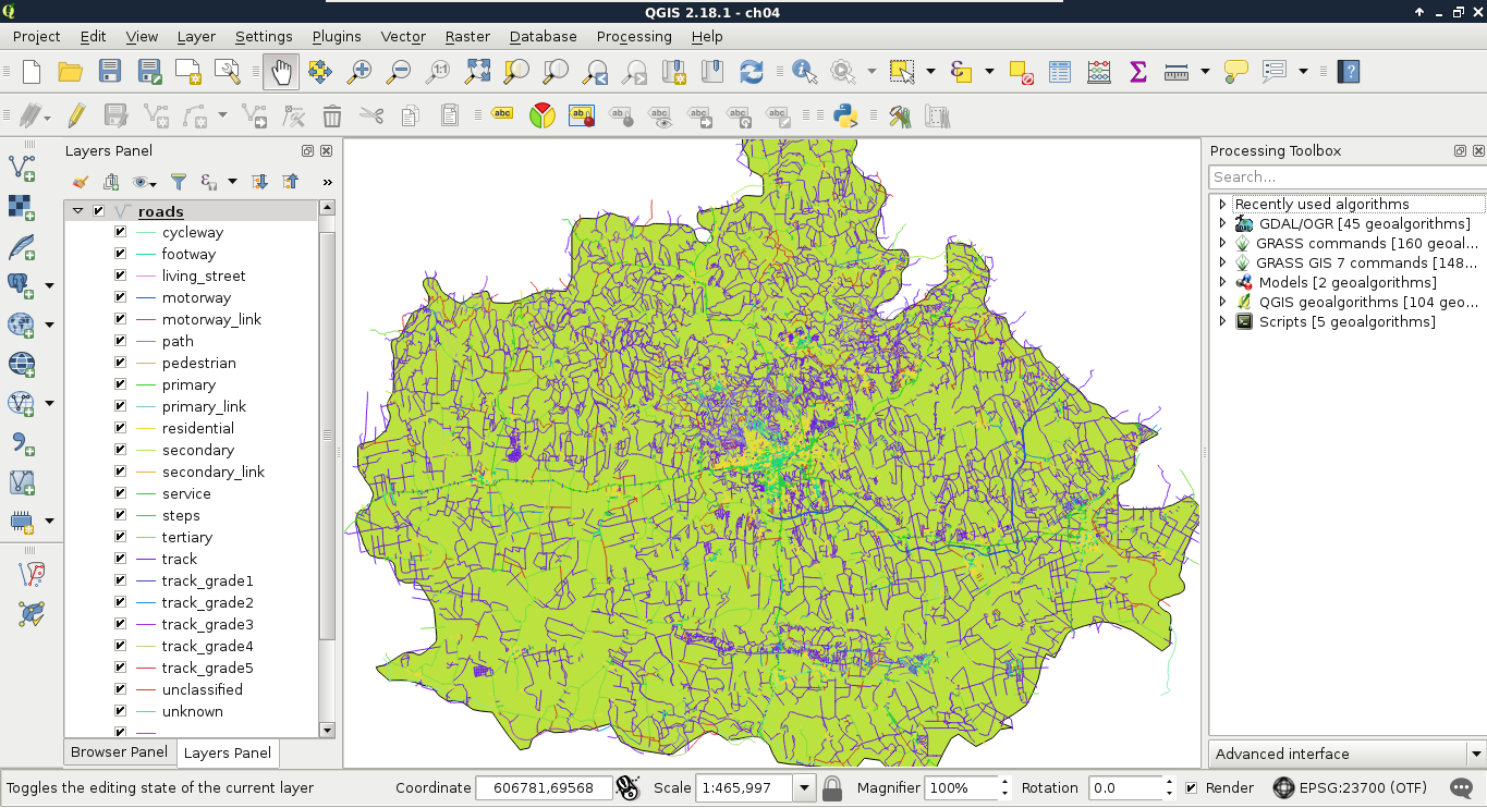
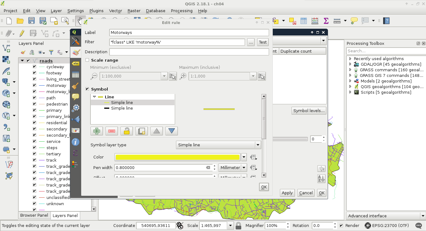
Furthermore, some of the classes belong to a single type. For example, the motorway and motorway_link classes distinguish between two subtypes of motorways. QGIS offers a great tool for these cases, called rule-based styling. Let's open the Style tab of our layer's Properties window, and choose Rule-based. We can remove the classification by selecting them all with the Shift key, and clicking on the minus button. For this scale, we will only show motorways, highways, and other important roads. We can add a rule with the plus button, which opens a dialog for creating a rule definition. By clicking on the ... button next to the Filter field, we can build our first definition as follows:

    "fclass" LIKE 'motorway%'

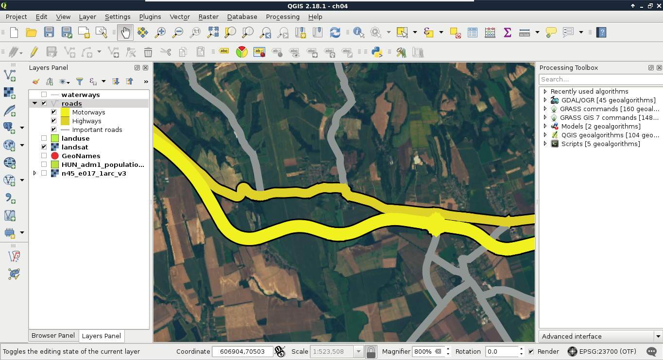
Similar to Google Maps, we create a complex line style for motorways, a thick yellow line with a thin black outline. We can do this by stacking two line styles. A 1 millimeter-wide black line goes to the bottom, while a 0.8 millimeter-wide yellow line goes on the top. This will create a 0.8 millimeter-wide yellow line with a 0.1 millimeter-wide black outline on both sides. First, we create the black line, then add a new line with the plus button. Finally, we style the new line:

The other roads should be styled following the same analogy, just with narrower lines. For selecting the highways, we can use the following query:

    "fclass" LIKE 'primary%'

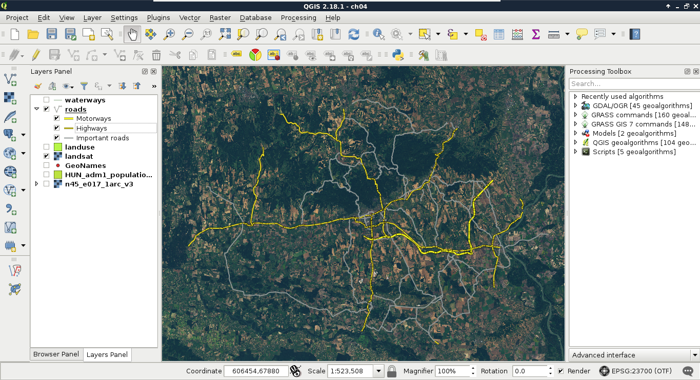
I visualized highways with a 0.6 millimeter-wide yellow line on a 0.8 millimeter-wide black line. Other important roads can be selected with a similar query:

    "fclass" LIKE 'secondary%'

For these roads, I created a single style, a 0.5 millimeter-wide grey line. By visualizing our roads on the top of the Landsat imagery, we can see our road map slowly getting in shape:

The only thing we lack is handling line connections properly. As we can see, our roads consist of several features. When those features connect, the ends of the lines are visible, and therefore, the whole image has a broken feeling. We can manipulate how those lines are rendered, though. As complex styles are rendered in different passes (layers), we can define their order. If we would like to create nice connections, we should render the black outlines first. As secondary roads are the least important, we should render them next. In the next pass, we should render highways, therefore, secondary roads connect into them directly, and only in the last pass we should render motorways. To define this order, we have to open the Symbol levels menu in our layer's Style tab. There, we just have to define the order with numbers. The higher the number, the later the style gets drawn.

If we create the ordering defined in this section, we get a more aesthetic result, as seen in the following screenshot: