Now that we have an appropriate suitability value, we can vectorize our suitability map. We've already seen how vector-raster conversion works, but we did not encounter raster-vector conversion. As every raster layer consists of cells with fixed width and height values, the simplest approach is to convert every cell to a polygon. GDAL uses this approach, but in a more sophisticated way. It automatically dissolves neighboring cells with the same value. In order to harness this capability, we should provide a binary layer with zeros representing non-suitable cells, and ones representing suitable cells:

1. Open a raster calculator, and create a binary layer with a conditional expression using the minimum suitability value determined previously. Such an expression is "suitability@1" >= 0.6. Save the result as a GeoTIFF file.
2. Open Raster | Conversion | Polygonize from the menu bar.
3. Provide the binary suitability layer as an input, and specify an output for the polygon layer:

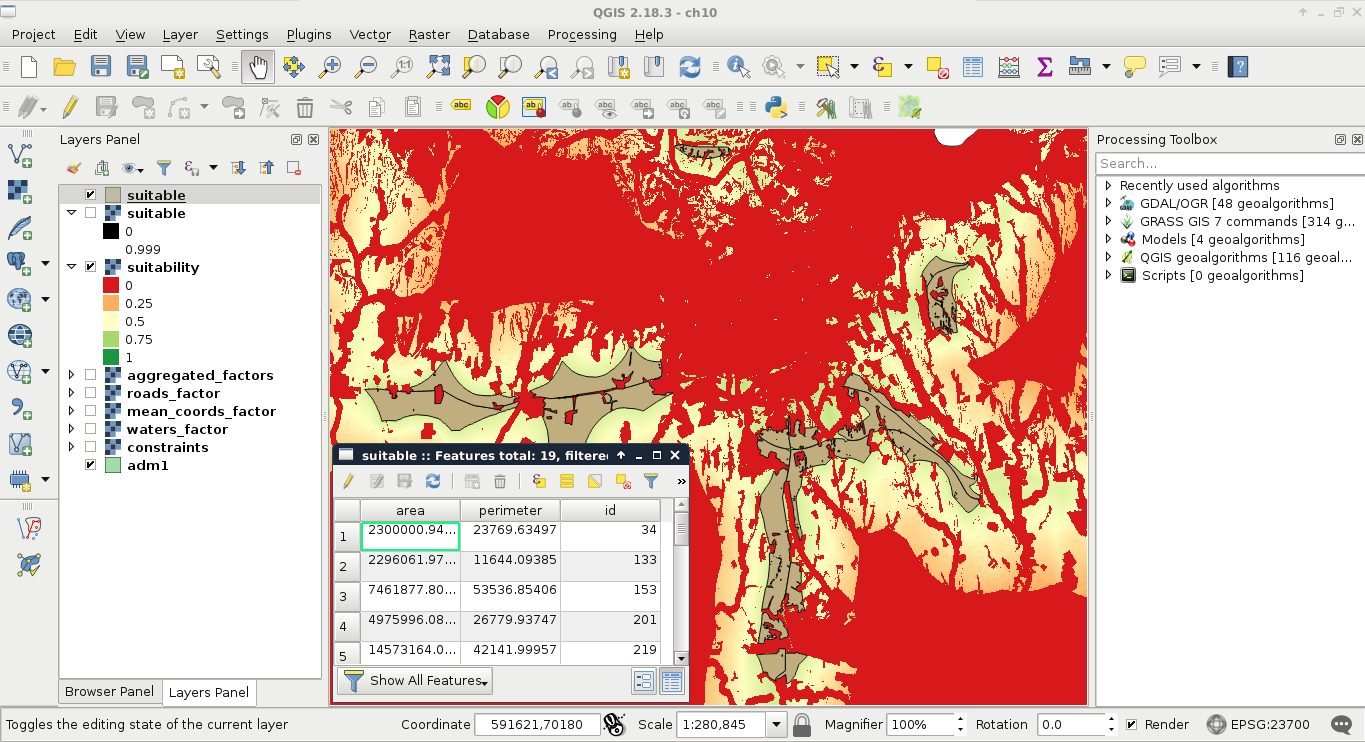
Now we have a nicely dissolved polygon layer with DN (digital number) values representing suitability in a binary format. We can apply a filter on the layer to only show suitable areas:

        "DN" = 1

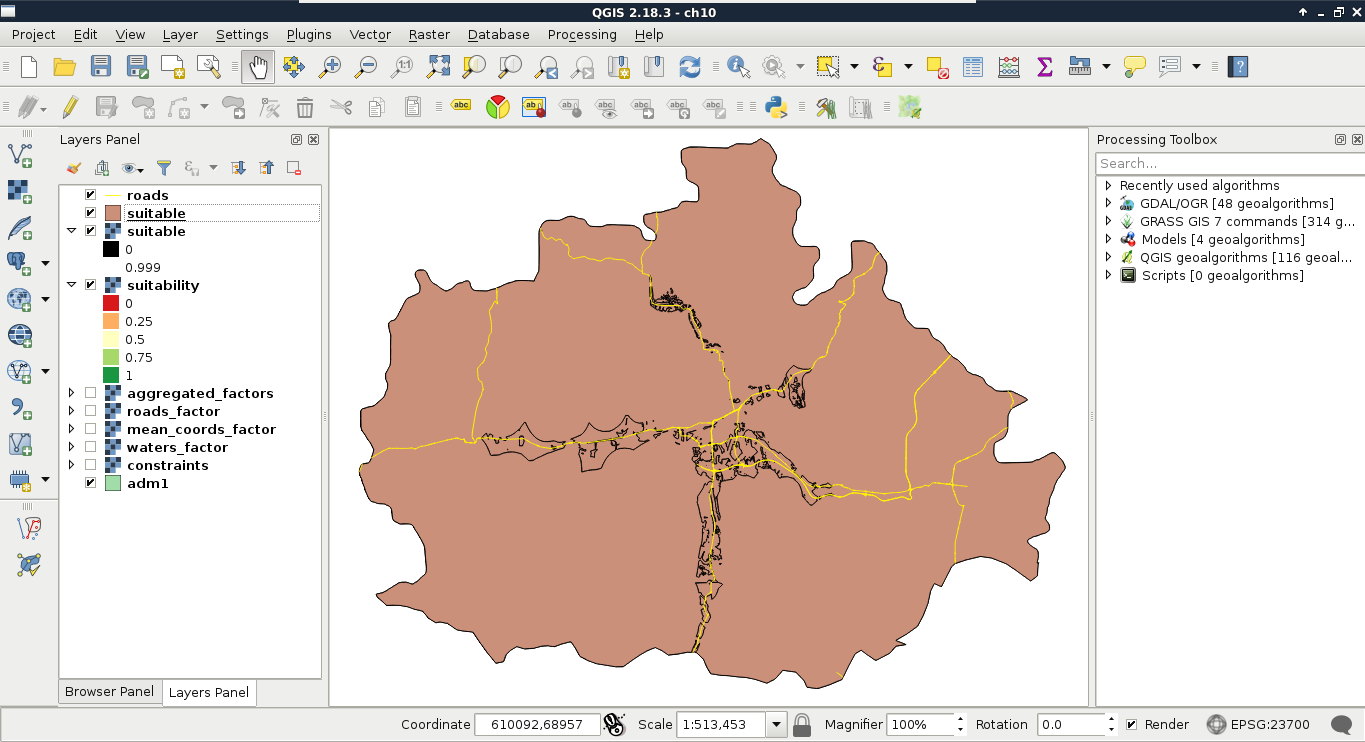
As the polygons do not respect the main roads, we need to cut them where the roads intersect them. This seems to be a trivial problem, although there are no simple ways to achieve this in QGIS. On the other hand, we can come up with a workaround, and convert our filtered polygons to lines, merge them with the roads, and create polygons from the merged layer.

4. Convert the filtered suitable areas layer to lines with QGIS geoalgorithms | Vector geometry tools | Polygons to lines. The output should be saved on the disk, as the merge tool does not like memory layers.
5. Merge the polygon boundaries with the roads layer by using QGIS geoalgorithms | Vector general tools | Merge vector layers. The output can be a memory layer this time.
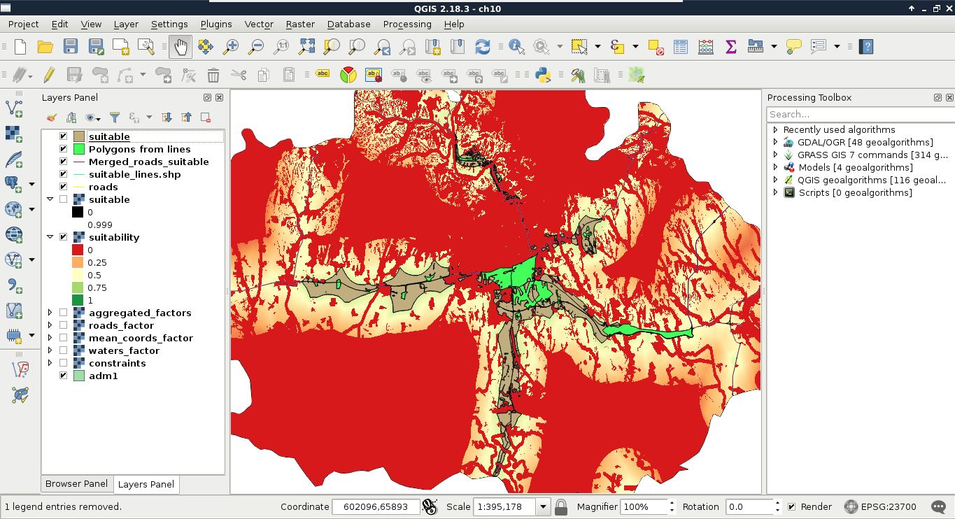
6. Create polygons from the merged layer with QGIS geoalgorithms | Vector geometry tools | Polygonize. Leave every parameter with their default values, and save the result as a memory layer.

7. Now we have our polygon layer split by the roads, however, we've also got some excess polygons we don't need. To get rid of them, clip the result to the original suitable areas layer with QGIS geoalgorithms | Vector overlay tools | Clip. Save the result as a memory layer.
8. Closely inspect the clipped polygons. If they are correctly split at the roads, and do not contain excess areas, we can overwrite our original suitable areas layer with this:

The last thing to do with our vector layer before calculating statistics is to get its attribute table in shape. If you looked at the attribute table of the polygonized lines, you would see that the algorithm automatically created two columns for the areas and the perimeters of the geometries. While we do not care about the perimeters in the analysis, creating an area column is very convenient, as we need to filter our polygons based on their areas. The only problem is that by clipping the layer, we unintentionally corrupted the area column. The other attribute we should add to our polygons is a unique ID to make them referable later:

1. Select the saved suitable areas polygon in the Layers Panel, and open a field calculator.
2. Check in the Update existing field box, and select the area column from the drop-down menu.
3. Supply the area variable of the geometries as an expression--$area, and recalculate the column.
4. Open the field calculator again, and add an integer field named id. The expression should return a unique integer for every feature, which is impossible to do in the field calculator. Luckily, we can access a variable storing the row number of every feature in the attribute table, which we can provide as an expression--$rownum.
5. Save the edits, and exit the edit session.

6. Apply a filter to only show the considerable areas using the expression "area" >= 1500000: