In order to create constraints, we need to convert our input features to raster maps. Before converting them, however, we need to open the correct layers, and apply filters on them to show only the suitable features:

1. Open the landuse layer and the SRTM DEM.
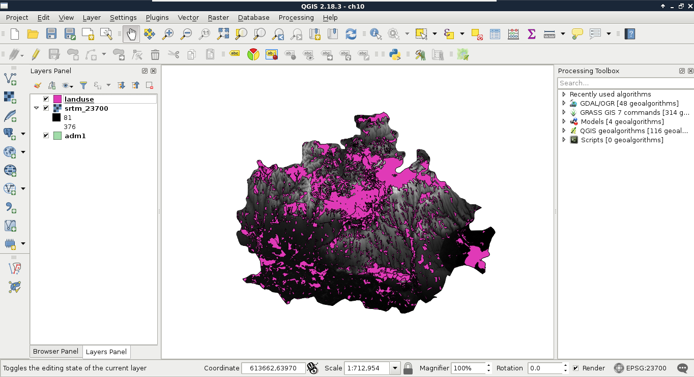
2. Apply a filter on the landuse layer to only show features which are restricted. It is simpler to create a filter which excludes land use types suitable for us, as we have fewer of them. Let's assume grass and farm types are suitable, as we can buy those lands. The only problem is that QGIS uses GDAL for converting between data types, which does not respect filtering done in QGIS. To overcome this problem, apply a filter on the layer with the expression "fclass" != 'grass' AND "fclass" != 'farm', then save the filtered layer with Save As:

The next step is to create the required raster layers. This step involves calculating slope values from the DEM, and converting the vector layers to rasters:

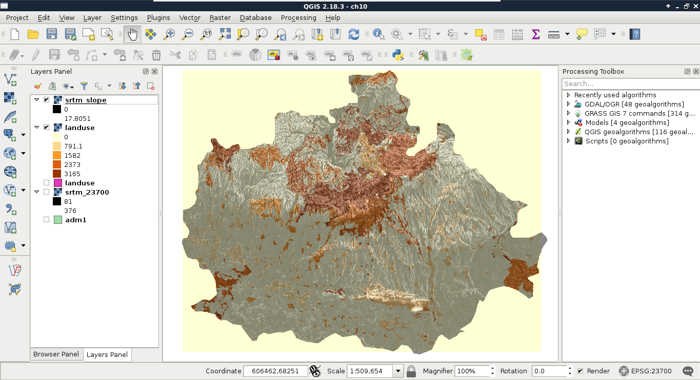
1. Calculate the slope values using Raster | Terrain Analysis | Slope from the menu bar. The input layer is the DEM, while the output should be in our working folder. The other options should be left with their default values.

2. Right-click on the DEM, and select Properties. Navigate to the Metadata tab, and note down the resolution of the layer under the Pixel Size entry. We could use more detailed maps for our vector features, however, as the resolution of our coarsest layer defines the overall accuracy of our analysis, we can save some computing time this way.
3. Convert the filtered land use layer to raster with the Raster | Conversion | Rasterize tool. The input layer should be the filtered landuse layer, the output should be in our working folder, while the resolution should be defined with the Raster resolution in map units per pixel option with the values noted down before. The attribute value does not matter, however, we should use absolute values for the resolutions. The order of the values noted down matches the order we have to provide them (horizontal, vertical).

4. Define our project's CRS on the resulting raster layer to avoid confusion in the future (Properties | General | Coordinate reference system):

Now we have a problem. Our land use raster's extent is limited to the extent of the land use vector layer. That is, the raster does not cover our study area. If we leave it like this, we instantly fail one of our criteria, as we do not analyze the whole study area. We can overcome this issue by creating a base raster. The Rasterize tool has an option to overwrite an existing raster, and burn the rasterized features in it:

1. Create a constant raster with QGIS geoalgorithms | Raster tools | Create constant raster layer. The reference layer should be the slope layer, as it covers the whole study area. The constant value should be 0. We can overwrite our land use raster with the output of this file.

2. Use the Rasterize tool again. The input should be the land use vector layer, while the output should be the constant raster we overwrote our land use raster layer with. We should keep the existing size and resolution this time (default option).

Now we have a continuous and a discrete raster layer, which should create a mask together somehow. Using vector data, we can easily overlay two layers, as both consist of the same types--geometries. We can compare geometries safely, and get geometries as a result. However, in case of raster data, the geometries are regular grids, and overlaying them makes little sense for any analysis. In this case, we overlay cell values which represent some kind of attribute. Considering this, how can we compare two completely different values? What can be the result of overlaying slope degrees and land use IDs? What is the intersection of 15° and 2831? The answer is simple--we can only get meaningful overlays from comparable layers. That is why we need to convert our slopes and land use to constraints--0% suitability and 100% suitability values.

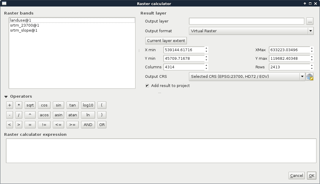
When we assign new values to raster layers based on some rules, it is called reclassification. We can reclassify raster layers in QGIS by using the raster calculator. Let's open it from Raster | Raster Calculator. The raster calculator in QGIS is somewhat similar to the field calculator, although it has limited capabilities, which include the following: 

• Variables: Raster bands from raster layers. Only a single band can be processed at a time, although we have access to different bands of multiband rasters by referencing their band numbers (for example, multiband@1, multiband@2, multiband@3, and so on).
• Constants: Constant numbers we can use in our formulas.
• Operators: Simple arithmetic operators, power, and the logical operators AND and OR.
• Functions: Trigonometric and a few other mathematical functions.
• Comparison operators: Simple equality, inequality, and relational operators returning Booleans as numeric values. That is, if a comparison is true, the result is 1, while if it is false, the result is 0:

With these variables, constants, and operators, we need to create a function or expression which iterates through every cell of a single, or multiple raster layers. The resulting raster will contain the results of the function applied to the individual cells. As our constraint maps should only contain binary values, we can get our first results easily by using simple comparisons as follows:

1. Reclassify the land use raster using the raster calculator. The rule is, every raster with an ID greater than zero should have the value of 0 (not suitable), while cells with zero values should get a value of 1 (suitable). We can use an expression like "landuse@1" = 0. The output should be a GeoTIFF file saved in our working folder.
2. Reclassify the slope raster using the raster calculator. We need every cell containing a slope value less than 10° to get a value of 1. Other cells should get a value of 0. The correct expression for this is "srtm_slope@1" < 10. Similar to the previous constraint, the output should be a GeoTIFF in our working folder:

Now we have two binary constraint layers, which can be directly compared, as their values are on the same scale. Using binary layers A and B, we can define the two simplest set operations as follows:

• Intersection (A × B): The product of the two layers results in ones where both of the layers have ones, and zeros everywhere else.
• Union (A + B - A × B): By adding the two layers, we get ones where any of the layers has a one. Where both of them have ones (in their intersections), we get twos. To compensate for this, we subtract one from the intersecting cells.

What we basically need is the union of constraints (zeros). Logically thinking, we can get those by calculating the intersection of suitable cells (ones). Let's do that by opening the raster calculator, and creating a new GeoTIFF raster with the intersection of the two constraint layers as follows:

    "landuse_const@1" * "slope_const@1"

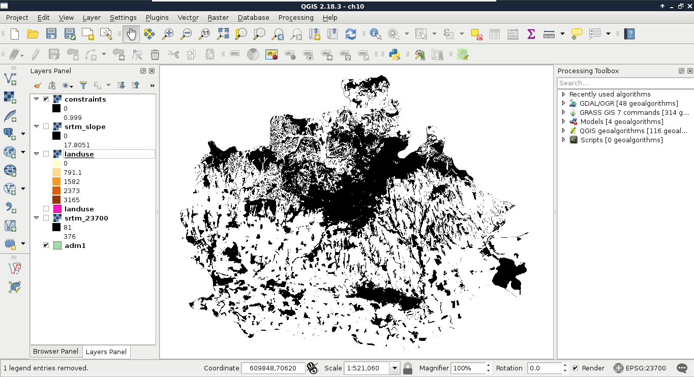
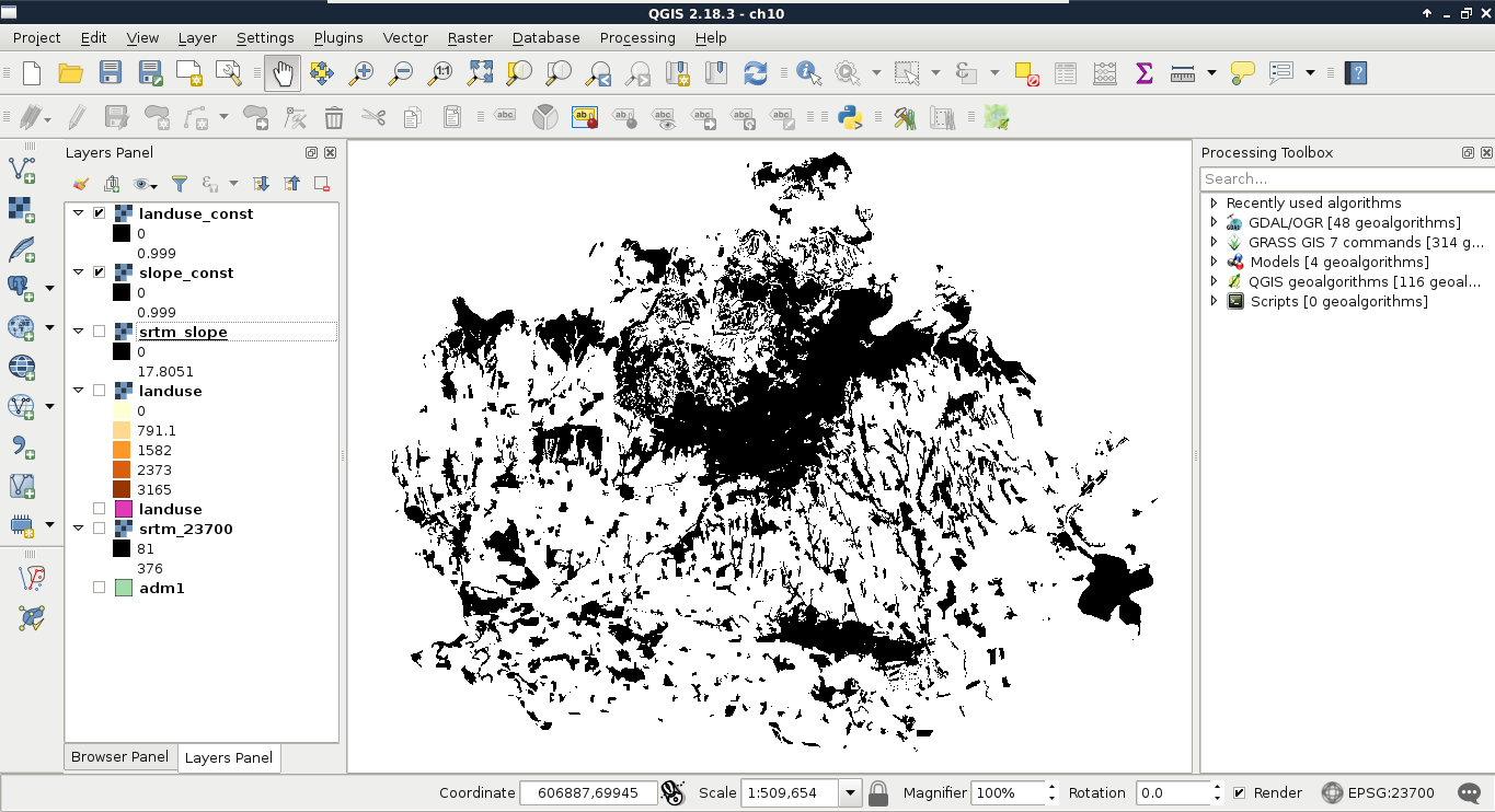
Now we can see our binary layer containing our aggregated constraint areas: