From the database and its schemas, we arrive at tables. As we know, databases can hold multiple schemas, while a single schema can hold multiple tables. Tables have typed columns and items as rows. What we did not discuss before is that tables can have a lot more properties. We can consider these constraints, rules, triggers, and indexes metadata, and we can set them with expressions, or from pgAdmin. If we inspect one of our tables, we can see the definition it was created with, which is as follows:

    CREATE TABLE spatial.adm1
    (
     id serial NOT NULL,
     geom geometry(Polygon,23700),
     name_1 character varying(75),
     hasc_1 character varying(15),
     type_1 character varying(50),
     engtype_1 character varying(50),
     population integer,
     popdensity double precision,
     pd_correct double precision,
     CONSTRAINT adm1_pkey PRIMARY KEY (id)
    )
    WITH (
     OIDS=FALSE
    );

If you've used an RDBMS before, this verbose CREATE TABLE expression resembles the usual ones; however, some of the lines are different. On the other hand, if we try to use a more regular expression, we end up with a similar table:

    CREATE TABLE spatial.test (
     id serial PRIMARY KEY NOT NULL,
     geom geometry(Point,23700),
     attr varchar(50)
    );

The first difference is that, in RDBMSs, keys are realized as constraints in the database. It is not just for keys, though. Almost every qualifier (except NOT NULL) is realized as a constraint. The most important qualifiers for tuning a database are NOT NULL, UNIQUE, PRIMARY KEY, and FOREIGN KEY. By adding the NOT NULL definition to a column, we explicitly tell PostgreSQL not to accept updates or new rows with an empty value for that field. Setting it for most of the columns is a good practice, as it can help to make the table more consistent. For example, it will prevent everyone from adding new features or updating existing ones without supplying the required attributes.

If we alter the spatial.test table created before with some updated definitions, we end up with two named constraints:

    ALTER TABLE spatial.test
     ADD UNIQUE (attr),
     ALTER COLUMN attr SET NOT NULL;

So far, we can see that PostgreSQL queries work in the concise way we might be used to. However, if we inspect the table in pgAdmin, it crafts more verbose, more explicit expressions to achieve the same results. We can also alter our tables in pgAdmin. We have to open the Properties of a table to reach the relevant options under the Columns and Constraints tabs. Under Columns, we can select any column, click on Change, and check the Not NULL checkbox in the Definition tab. For setting the unique constraint, we have to add a new, Unique item in the Constraints tab. In the dialog, we only have to provide the column name in the Column tab, and click on Add:

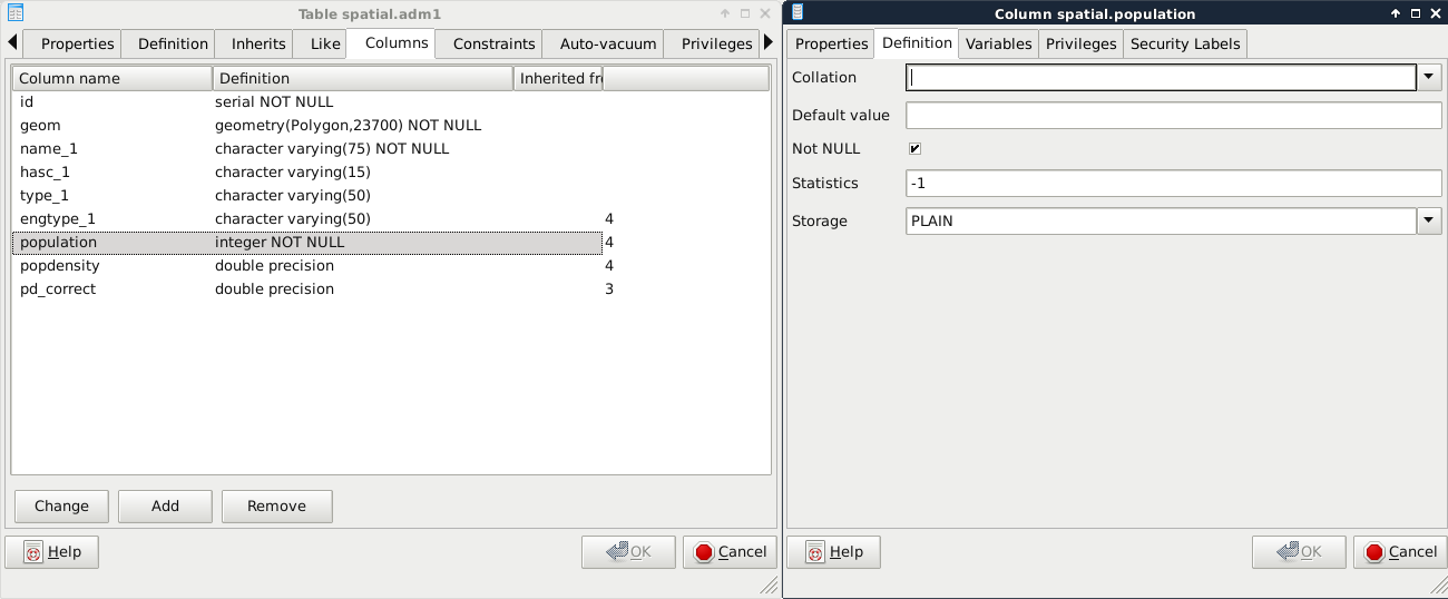
The last constraint we should explore is CHECK. We can create rules that the columns have to comply with before an update or insert occurs by using regular SQL expressions. For example, we can create a CHECK for the population column, and use the population > 0 expression to enforce a positive population value. Another reason to use a CHECK constraint is to validate the geometries themselves, as PostGIS only checks that they are using the right geometry type. For this task, we have to create a CHECK, as we would add a UNIQUE definition:

1. In one of the spatial tables' Properties window, select the Constraints tab.
2. Add a new Check.
3. In the Definition tab, supply the following expression--ST_IsValid(geom):

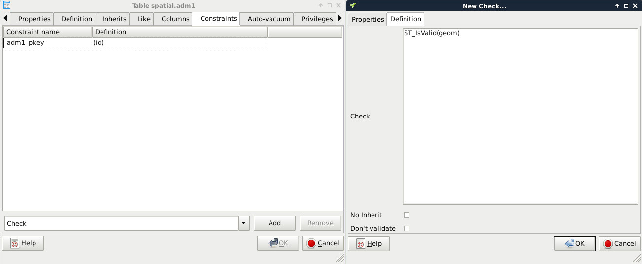
If we look at the SQL tab, we can see that defining a CHECK is very similar to defining other constraints with an expression:

    ALTER TABLE spatial.adm1
     ADD CHECK (ST_IsValid(geom));

Let's see a real world example. PostGIS has the capability to handle curves. Besides the regular points, lines, polygons, and their multipart counterparts, PostGIS handles the following geometry types:

• Triangle: A simple triangle
• Circular String: A basic curve type, which describes a circular arc with two end points and minimum of one additional point on the circle's perimeter
• Compound Curve: A geometry mixing line strings and circular strings
• Multi Curve: The multipart geometry mixing line strings, circular strings, and compound curves
• Curve Polygon: A polygon-like geometry, although the polygon can be made of line strings, circular strings, and compound curves
• Multi Surface: A multipart geometry mixing regular polygons and curve polygons
• Polyhedral Surface: A surface made of polygons--useful for storing 3D models.
• TIN (Triangulated Irregular Network): A surface made of triangles--useful for representing Digital Elevation Models (DEM) with vector data

Sometimes, we would like to store curves to have a representation which can be visualized instantly without post-processing. Unfortunately, there is no function in PostGIS which smoothes lines with a nice smoothing algorithm. To fill this gap, I created a small and primitive script, which converts corners to curves based on some rough approximations. First of all, let's get this script (createcurves.sql) from the supplementary material's ch07 folder, or download directly from https://gaborfarkas.github.io/practical_gis/ch07/createcurves.sql. We can open the file in pgAdmin's SQL window, and run the content as a regular SQL expression. When we are done, we should have access to the CreateCurve function.

In this example, we will build a table storing the curvy representation of our rivers table. First of all, we need to create a table which will contain our curves. We could save the results of a query directly into a table; however, we will also apply some logic, which is as follows:

• Only the IDs and the geometries get stored.
• PostGIS must only accept compound curves as geometries, as our custom function can only return compound curves when fed with line strings.
• The IDs reference the IDs of the original table. If we delete a row from the original waterways table, PostgreSQL must also delete its curvy representation.
• If we update the original table, PostgreSQL must automatically update the curve table accordingly.

We can apply some of this logic when we create the table with the correct table definition in an SQL window as follows:

    CREATE TABLE spatial.waterways_curve (
     id integer PRIMARY KEY UNIQUE REFERENCES spatial.waterways (id)
     ON DELETE CASCADE,
     geom geometry(CompoundCurve, 23700)
    );

With this preceding definition, we defined two columns: one for the IDs, and one for the geometries. The IDs are foreign keys, as they reference another column in another table. By adding the ON DELETE CASCADE definition, we ask PostgreSQL to delete referencing rows from this table when rows get deleted from the parent table. The geometry is defined as compound curves in our local projection (the number should reference your local SRID). This table definition alone fulfilled some of our requests. There is a great feature in PostgreSQL which we can apply to the rest of them--rules.

Before creating the rules, we should synchronize our new table with the waterways table. We can insert values into an existing table with the INSERT INTO expression. What is more exciting is that we can shape a SELECT statement to insert the results instantly into a destination table as follows:

    INSERT INTO spatial.waterways_curve (
     SELECT id, CreateCurve(geom) FROM spatial.waterways
    );

Rules are custom features of PostgreSQL, which allow us to define some logic when we select, update, delete, or insert rows in a table. In a rule, we can define if we would like to apply our custom logic besides the original query, or instead of it. In order to define a rule, we can select our waterways table in pgAdmin, right-click on Rules, and select New Rule:

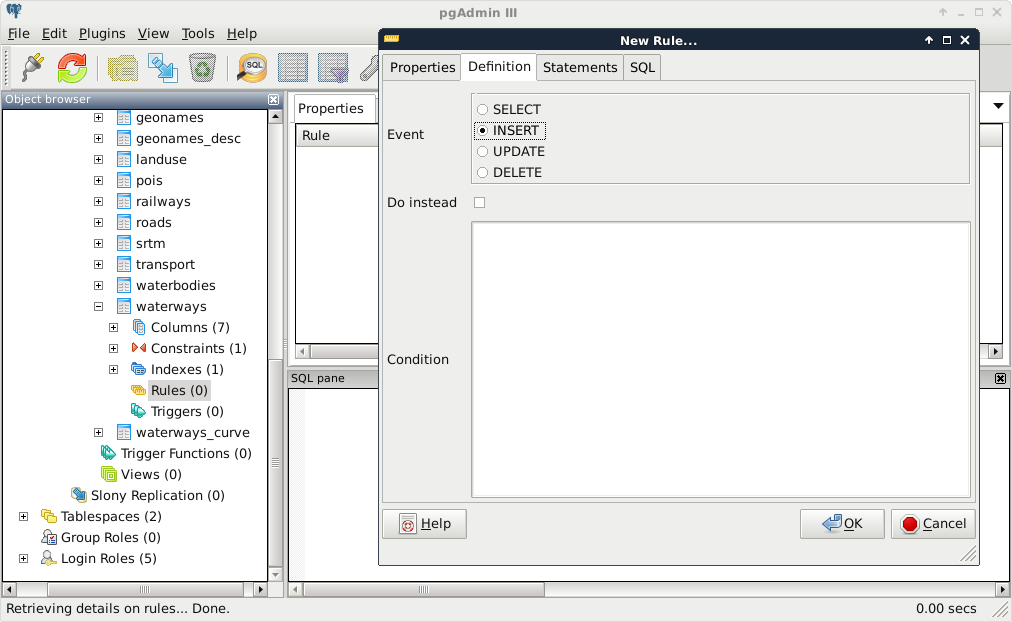
The rule maker of pgAdmin is a little bit scattered, as rules are quite complex. There are these three distinct tabs we need to fill in order to have a rule:

• The first thing we can define is the rule's name in the Properties tab (for example, waterways_insert).
• In the Definition tab, we can define the event we would like to hook our rule onto. Rules are like event listeners in object-oriented languages. They are invoked when an event we hooked them onto occurs. We should select INSERT for our first rule. We can also supply a condition, which has to happen in order to run the rule. We can leave that field empty.
• The Statements tab holds the body of our rule. Every logic we would like to execute when our event triggers goes there. As we need PostgreSQL to automatically generate curves from new geometries, we can insert some of the new row's values into the curve table directly:

    INSERT INTO spatial.waterways VALUES (
     NEW.id, CreateCurve(NEW.geom)
    );

As we are now inserting literal values directly into a table, we have to provide the VALUES keyword. Other RDBMSs might also require us to provide the columns we would like to insert our values into; however, PostgreSQL is smart enough to find out that we only have two columns in the new table with matching types. There is one additional thing we need to keep in mind when writing rules and triggers--row variables. We can access the processed rows with the keywords NEW and OLD. Of course, we should only use the appropriate one from the two. That is, if we write a rule for an INSERT, we should use NEW. If we write a rule for an  UPDATE, we can use both of them, while for DELETE events, we should only use OLD.

The second rule should occur when we update the waterways table. In this case, we should only update the curve table when a geometry changes; therefore, we need a condition besides the rule body:

1. Name the rule in the Properties tab.

2. Select the UPDATE event in the Definition tab, and add the following expression as a Condition--NOT ST_Equals(OLD.geom, NEW.geom).
3. Write the rule's body in the Statements tab as follows:

    UPDATE spatial.waterways_curve SET geom = CreateCurve(NEW.geom)
     WHERE id = NEW.id;

As you can see, we can directly compare the new and old values of the updated row, but PostgreSQL has no idea how it should update the curve table. Therefore, we have to supply a WHERE clause defining where we would like to update our geometry if it differs from the old one. Of course, we can also use OLD.id, as the two should be the same.

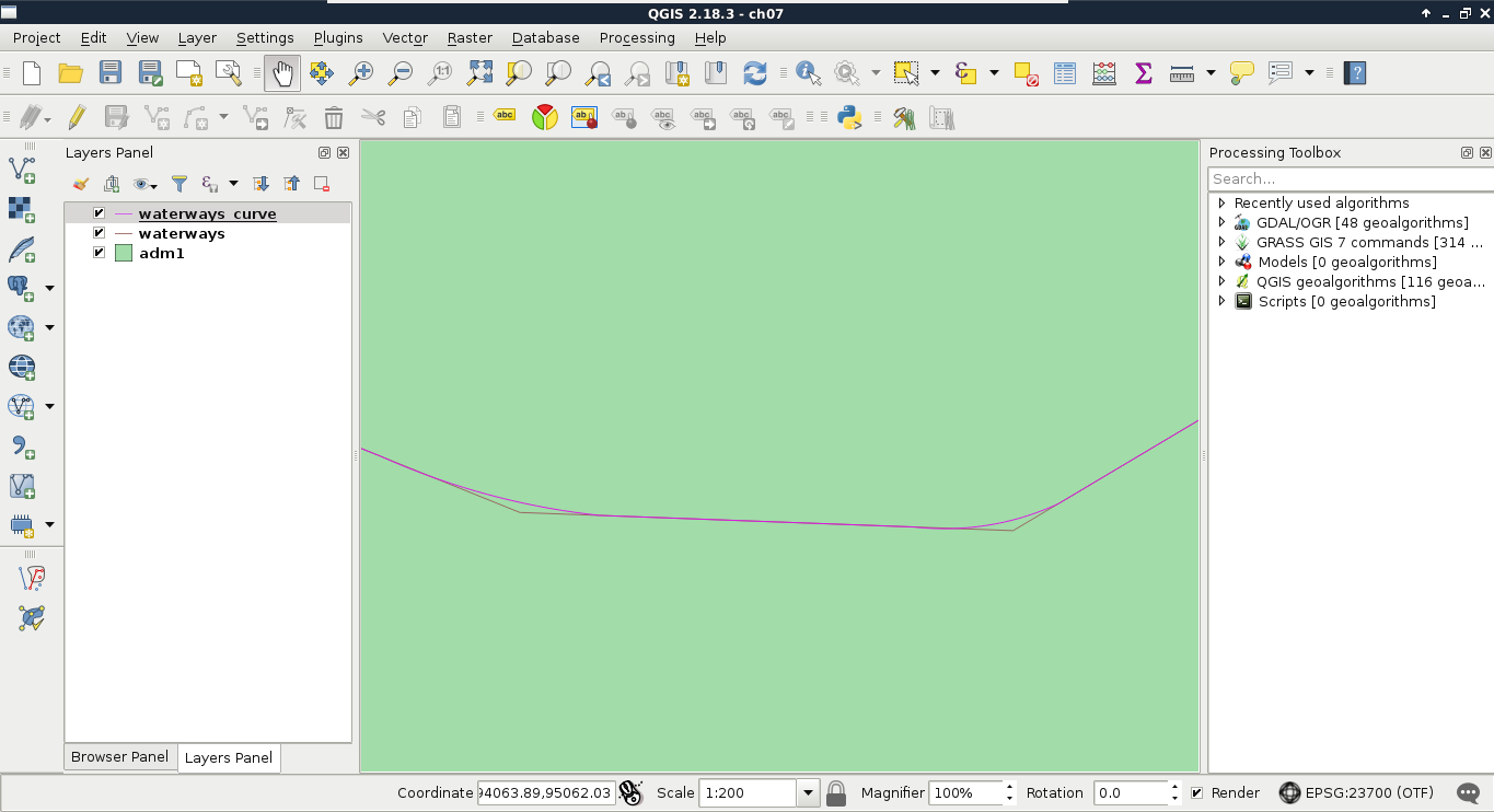
We don't have to create a rule for deleting rows, as the cascading constraint on the foreign key will make sure that the rows deleted from the waterways table get deleted from the curve table. Let's see, instead, what we created in QGIS. First of all, we can see in the database manager that QGIS recognizes the compound curves we have as line geometries, as it also supports circular strings. If we open the layer, and zoom in to a corner, we can see our curves:

To check if everything works as expected, we have to edit our waterways table a little bit, in the following way:

1. Select the waterways layer in the Layers Panel.
2. Start an edit session with the pencil-shaped Toggle Editing button in the main toolbar.
3. Select the Node Tool from the freshly enabled tools in the main toolbar.
4. Click on one of the lines, and move one of its vertices a little bit with the red anchor.
5. Save the edit by clicking on the Save Layer Edits button.
6. Refresh the layers by panning, zooming, or clicking on the Refresh button in the main toolbar.

If everything is configured properly, we should be able to see our curve layer following the edits we made in the waterways layer. The only problem left is that we can update the curve table manually, getting the tables out of synchronization. We can easily avoid this, however, by smart permission control. What do we know about rules? Only table owners can define them on tables; therefore, PostgreSQL will run them on behalf of the owner. Thus, we can fine-tune the privilege system in the following way:

1. Set the curve table's owner to a superuser role, like postgres.
2. Set the waterways table's owner to a superuser role, like postgres.
3. Give select privilege to the GIS role on the curve table with the expression GRANT SELECT ON TABLE spatial.waterways_curve TO gis;.
4. Give every privilege to the GIS role on the waterways table with the expression GRANT ALL ON TABLE spatial.waterways TO gis;.

Now we can modify the waterways table with the GIS role, but only the postgres superuser can modify the curve table. That is, we can only access the curves layer with the GIS role, but the rules we defined change the curve table accordingly and automatically when we modify the waterways table.