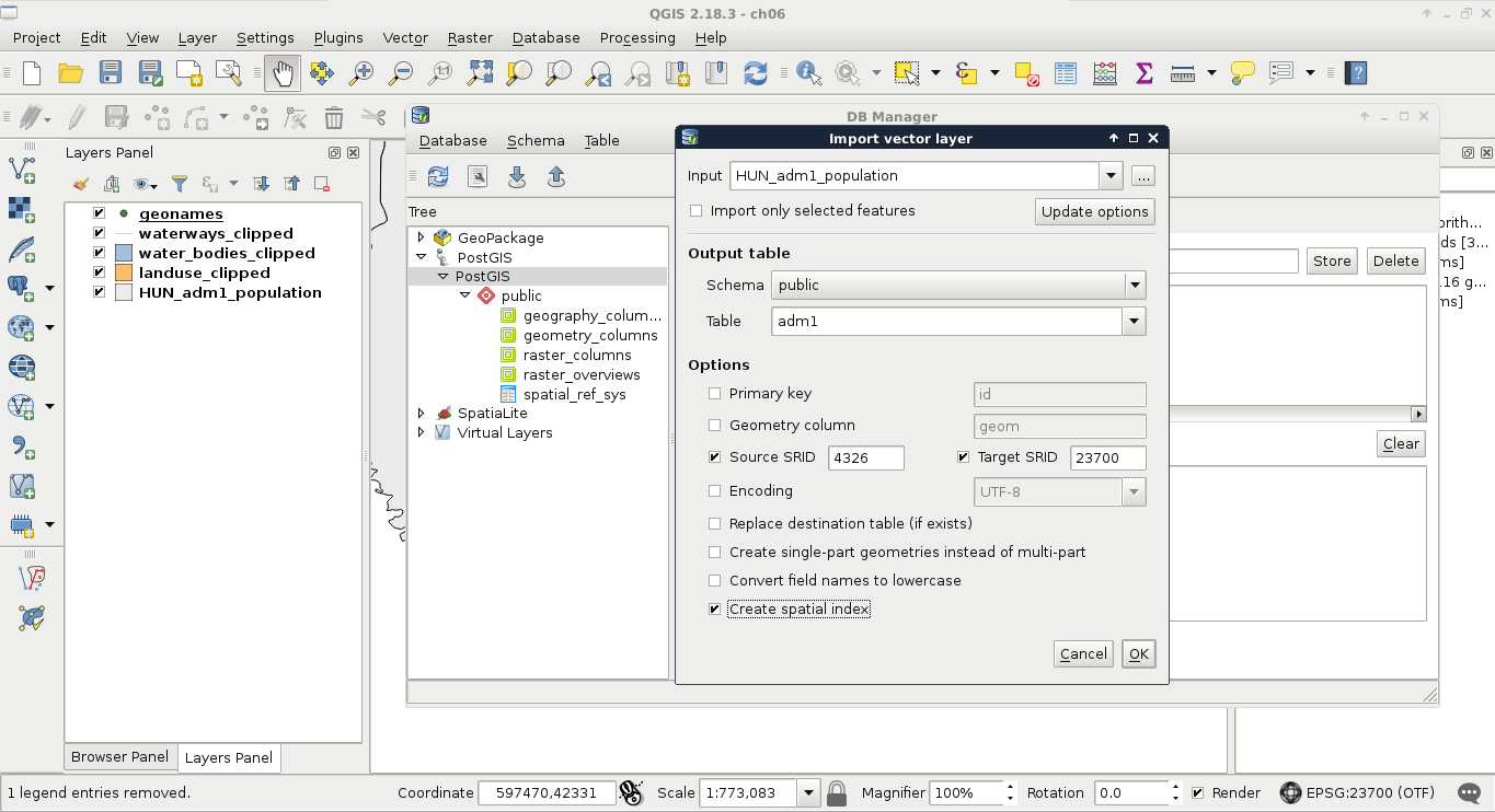
First of all, let's load the two layers saved on the disk--the GeoNames and the administrative boundaries layers. We can import layers with the Import layer/file button accessed from QGIS's database manager. QGIS automatically converts the specified layer to a PostGIS table by providing the required properties. We can import virtually any vector layer with the following steps:

1. Choose the input layer in the Input field. We can also specify layers not loaded in QGIS with the browse button (...) next to the field.
2. Choose a Schema to load the layer into. In our case, the public schema is the only one available.
3. Provide a table (PostGIS layer) name in the Table field.
4. Define the source and target projections. It can be omitted if you would like to keep the current projection. Let's save the layers in the local projection you're using by using 4326 as Source SRID and your local projection's EPSG code as the Target SRID (without EPSG).
5. Check the Create spatial index box. Consider the following screenshot:

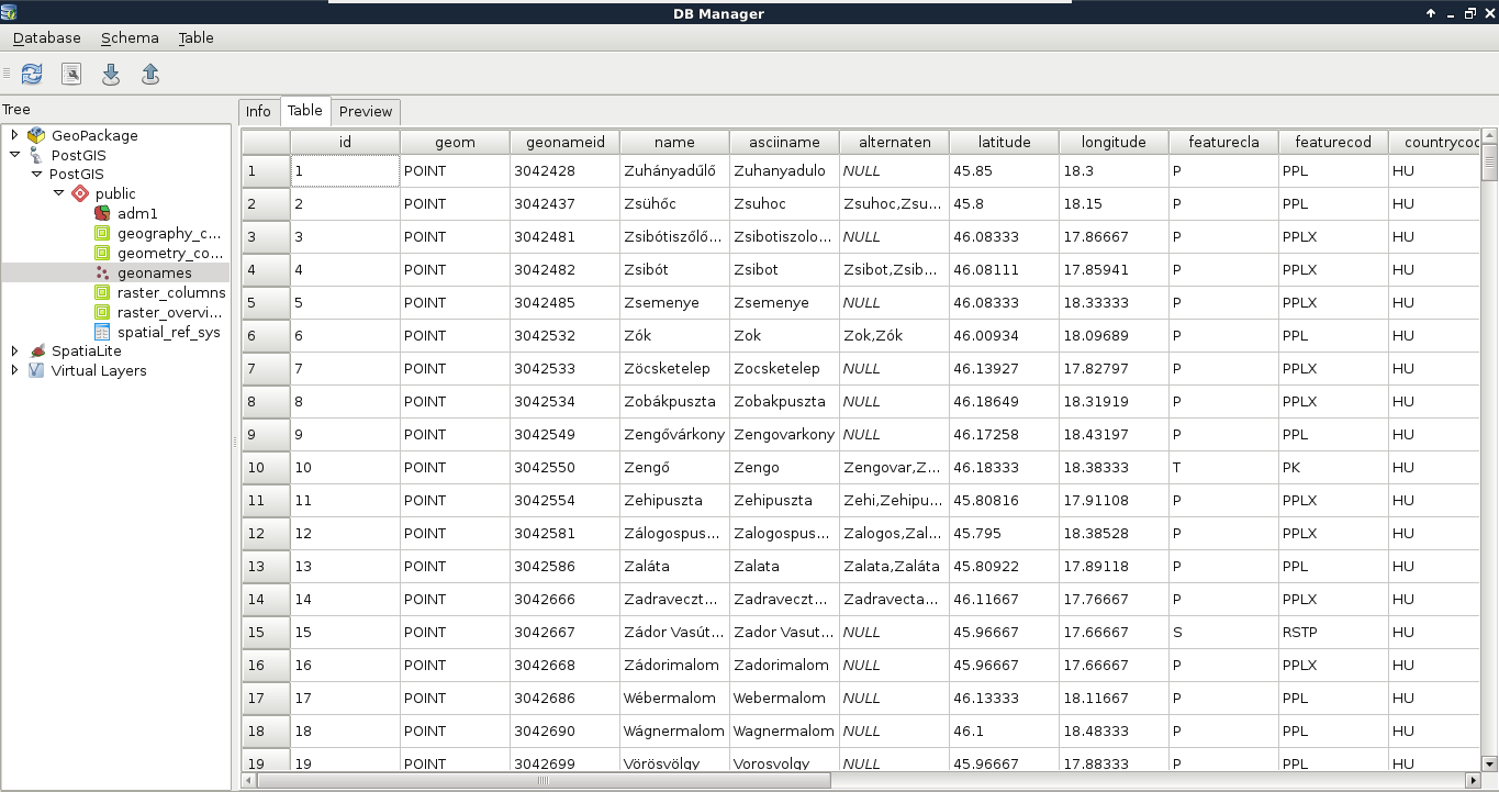
If we reconnect to the database, we can see the two imported tables. We can inspect them by clicking on them and navigating to the Table and Preview tabs. If we inspect the values stored in the tables, we can conclude that every value is loaded successfully. We have null values, integers, floating point values, and strings. The only problem is that we cannot define which columns we would like to import. If we delete the columns within QGIS, we would lose them also on the disk. Luckily, we can run the SQL queries within QGIS's database manager and drop the excessive columns manually:

6. By opening the SQL window, we can build an SQL expression for dropping columns. It does not matter what layer we selected as we must provide the table to remove columns from. The syntax for dropping columns looks like the following:

        ALTER TABLE tablename DROP COLUMN column1,
         DROP COLUMN column2, etc.;

Therefore, to drop the id_1, name_0 and iso columns of the adm1 layer, we can run the following expression:

        ALTER TABLE adm1 DROP COLUMN id_1, DROP COLUMN name_0,
         DROP COLUMN iso;

We had an easy task importing two basic layers into PostGIS--one with point geometries and one with polygon geometries. What happens when we have layers with mixed geometry types? Of course, mixing points, lines, and polygons are strongly discouraged, but mixing single and multipart geometries of the same type is a common thing. The only problem is that PostGIS doesn't allow us to do so.

7. Let's try to import our in-memory waterways layer:

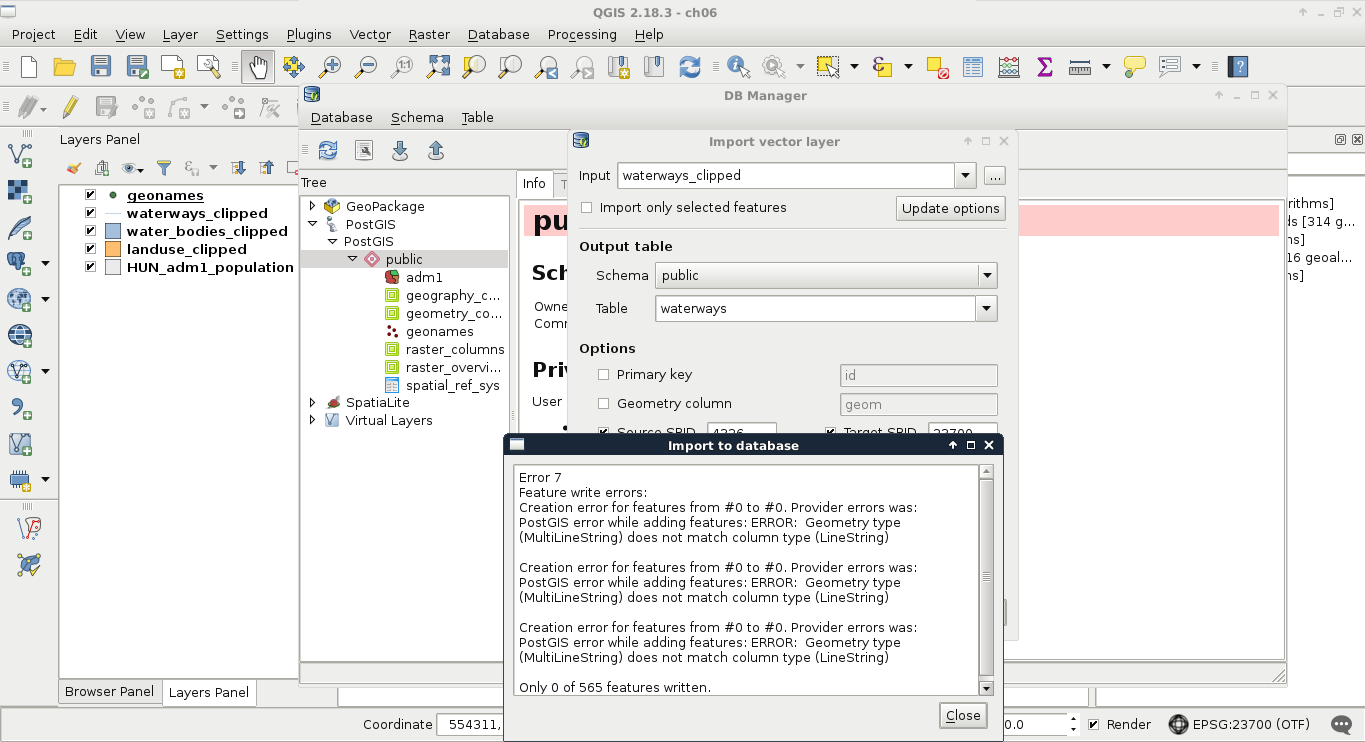
No matter how we try to import, if we have mixed geometry types, we end up with an error. Our layer has line string and multipart line string geometries mixed, while PostGIS only accepts one of them. The solution is simple though. We either have to explode multipart geometries or convert single geometries to multipart ones based on an attribute. Although we would get a little more optimal result if we stick with the lowest common denominator (in this case, multipart geometries), QGIS does a poor job in doing it. To convert our features to multipart geometries, we would need a column with duplicated values, therefore, we would lose data. As this is not an ideal solution, we have to convert our layer to single-part geometries, duplicating some of the data.

8. We can use QGIS geoalgorithms | Vector geometry tools | Multipart to singleparts from the Processing toolbox to achieve this. The output should be a memory layer (memory:):

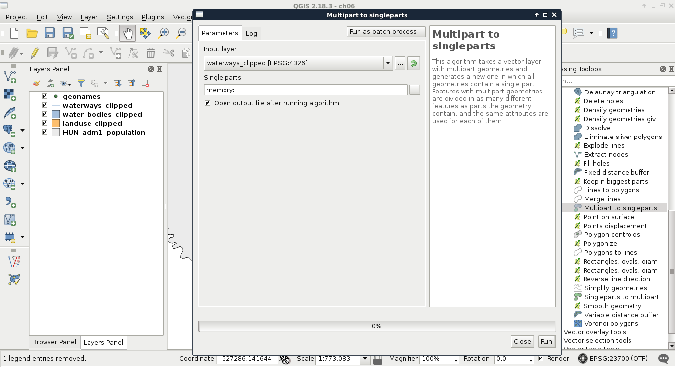
Now we can upload the resulting layer to PostGIS with the previous steps. If we put these steps and considerations together, we end up with this workflow to import every layer we need into PostGIS:

1. Clip the vector layer to the study area if it is not clipped already. Of course, you can import the whole layer but doing so will have a performance hit.
2. Try to import the layer to PostGIS. If you have mixed geometries, the import will fail.
3. Convert the multipart geometries to single part with the Multipart to singleparts tool. You can achieve the same with other tools; don't be afraid to experiment.
4. Import the new layer to PostGIS. Don't forget to check the Replace destination table (if exist) checkbox as if you have a failed attempt to create a table, an empty table will remain there. The problem is it may have the wrong geometry type.

We will need the following layers added to the PostGIS database:

• The whole administrative boundaries layer
• The clipped GeoNames, water ways, water bodies, and land use layers
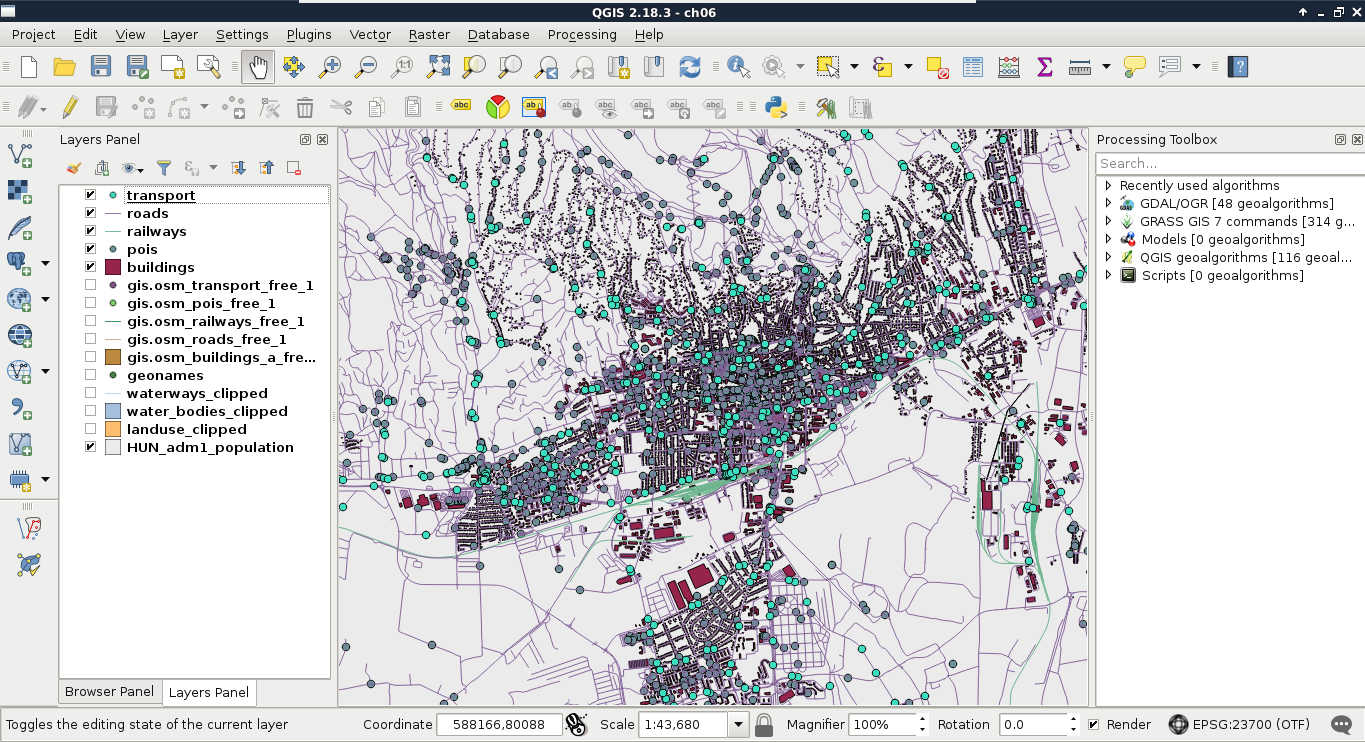
• The OSM (OpenStreetMap) layers we did not bother with or process before: the road layer (gis.osm_roads_free_1.shp), the railways layer (gis.osm_railways_free_1.shp), the buildings layer (gis.osm_buildings_a_free_1.shp), the POIs layer (gis.osm_pois_free_1.shp), and the transport layer (gis.osm_transport_free_1.shp)

Now that we have a bunch of layers we did not clip or alter too much to import, we need an effective way to process them. First of all, we need to decide if we would like to add them to the canvas before processing. If we do so, we can spare the overhead time of reading in the layers and furthermore, build spatial indexes on them to speed up the clipping process. We can also leave them on disk and spare some clicks. Either way, let's apply the usual filter on our administrative boundaries layer and open the Clip tool from QGIS geoalgorithms | Vector overlay tools.

In the clipping tool, we can access batch processing by clicking on the Run as batch process button. There we can create as many rows as we need for processing each layer with minimal hassle. Now we face another dilemma. We can save every result as a memory layer, although we cannot name them. Therefore, we need to distinguish between the results manually. Fortunately, it isn't that hard in our case as we have one polygon layer, two line layers with very different densities, and two point layers:

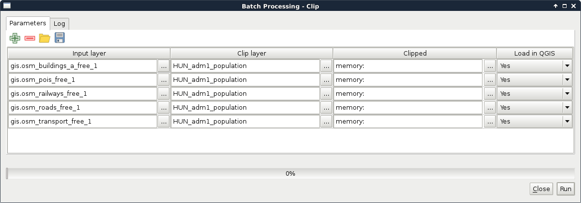
To distinguish between the two point layers, we can toggle the visibility of the original layers and the clipped layers and compare them visually. After guessing the names of the layers correctly, we can proceed and load them into PostGIS following the previous steps: