Although calculating statistics from a whole raster layer has its own advantages, now we need raster statistics from only the portions overlapping with our suitable areas. We can do this kind of calculation automatically by using zonal statistics. Zonal statistics require a raster layer and a polygon layer as inputs, then creates and fills up attribute columns with all kinds of statistical indices (like count, sum, average, standard deviation, and so on) in the output polygon layer. In order to calculate all the required statistics, we need all the input raster layers first:

1. Open every raster layer needed for the statistics--the water distance, the mean coordinate distance, the slope, and the suitability layers.
2. Open the Raster | Zonal statistics | Zonal statistics tool. 

3. Choose an appropriate raster layer as Raster layer, the suitable areas layer as the Polygon layer containing the zones, and supply a short prefix describing the raster layer (for example, mc_ for mean coordinates). Save the result as a memory layer. Check the appropriate indices, and uncheck the rest of them. Remember, water distance--minimum; mean coordinates--average (mean); slope--minimum, average, maximum; suitability--minimum, average, maximum.
4. Repeat the process for every input raster layer:

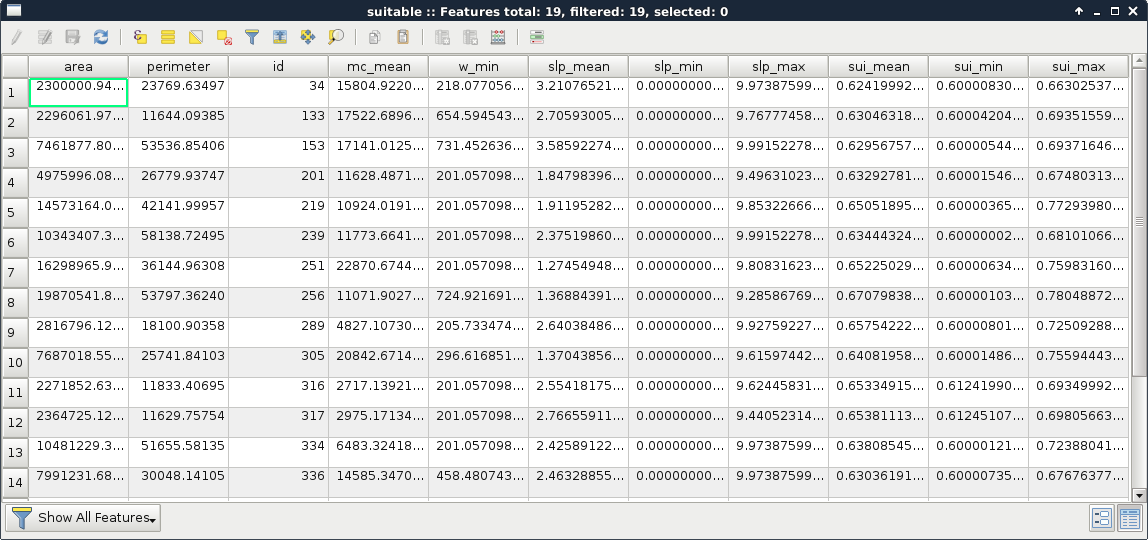
That's all. With a few clicks, we can get a lot of statistical indices from different raster layers and some polygons. On the other hand, those numbers are not comprehensive at all. For example, we do not know about the distribution of suitability values from some indices. As a matter of fact, having a histogram of the suitability values could enhance decision making, as we would see how common less suitable values, and the more suitable values in a site are. For that, we would need the histogram of the raster layer under our potentially suitable areas. Unfortunately, creating zonal histograms is not available in QGIS. Furthermore, the easiest approach involves a lot of manual labor. Let's create one or two histograms just to get the hang of it:

1. Open the attribute table of the suitable areas, and select the first row by clicking on the row number on the left.
2. Save the selected feature using Save As, and specifying Save only selected features.
3. Use the Clipper tool to clip the suitability raster layer to the saved feature.
4. Copy the style of the suitability layer, and paste it on the clipped suitability layer (this way, we get a colored line in the histogram).
5. Open Properties | Histogram on the clipped raster, and save the histogram as a PNG file with the Save plot button. Use the ID of the selected feature in the file name (for example, histo_34.png).

There are still several problems with this approach, although this is the closest we can get to a histogram in QGIS without scripting in Python or R. The problems include the following:

• The values are not binned. We have every different value as a single interval, making the histogram noisy.
• The frequency is expressed in cell counts. It would be much more clear if the frequency would be expressed in percentage values.