We can not only select features by their attributes, but also by their spatial relationships. These queries are called spatial queries, or selecting features by their location. With this type of querying, we can select features intersecting or touching other features in other layers. The most convenient mode of spatial querying allows us to consider two layers at a time, and select features from one layer with respect to the locations of features in the other one. First of all, let's remove the filter from our GeoNames layer. Next, to access the spatial query tool in QGIS, we have to browse our Processing Toolbox. From QGIS geoalgorithms, we have to access Vector selection tools and open the Select by location tool:

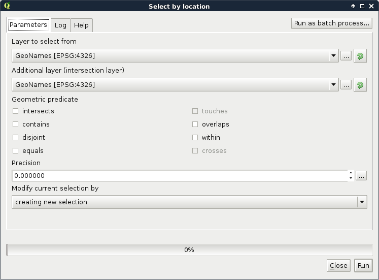
As we can see, QGIS offers us a lot of spatial predicates (relationship types) to choose from. Some of them are disabled as they do not make any sense in the current context (between two point layers). If we select other layers, we can see the disabled predicates changing. Let's discuss shortly what some of these predicates mean. In the following examples, we have a layer A from which we want to select features, and a layer B containing features we would like to compare our layer A to:

• Intersects: Selects every feature from A which intersects any feature in B.
• Contains: Selects every feature from A which contains (fully encapsulate) any feature in B.
• Disjoint: Selects every feature from A which does not intersect any feature in B (inverse of intersects).
• Equals: Selects every feature from A which can be also found in layer B (can be used to check for duplicates, that is, if A and B are the same).
• Touches: Selects every feature from A whose boundary intersects the boundary of any feature in B, but not its interior. The interior and boundary of a point are the same, while in a line string, the boundary consists of the two nodes (end points) and the interior is everything between them.
• Within: Selects every feature from A which is contained (fully encapsulated) by any feature in B.

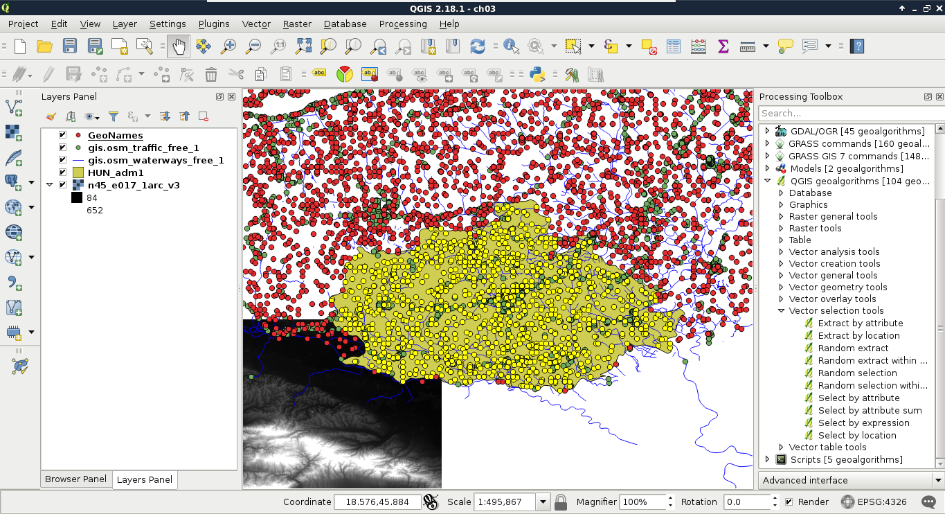
Let's select every feature from the GeoNames layer in our study area. As we have our study area filtered, we can safely pass the administrative layer as the Additional layer parameter. The only thing left to consider is the spatial predicate. Which one should we choose? You must be thinking about intersects or within. In our case, there is a fat chance that both of them yield to the same result. However, the correct one is intersects, as within does not consider points on the boundary of the polygon. After running the algorithm, we should see every point selected in our study area. Consider the following screenshot:

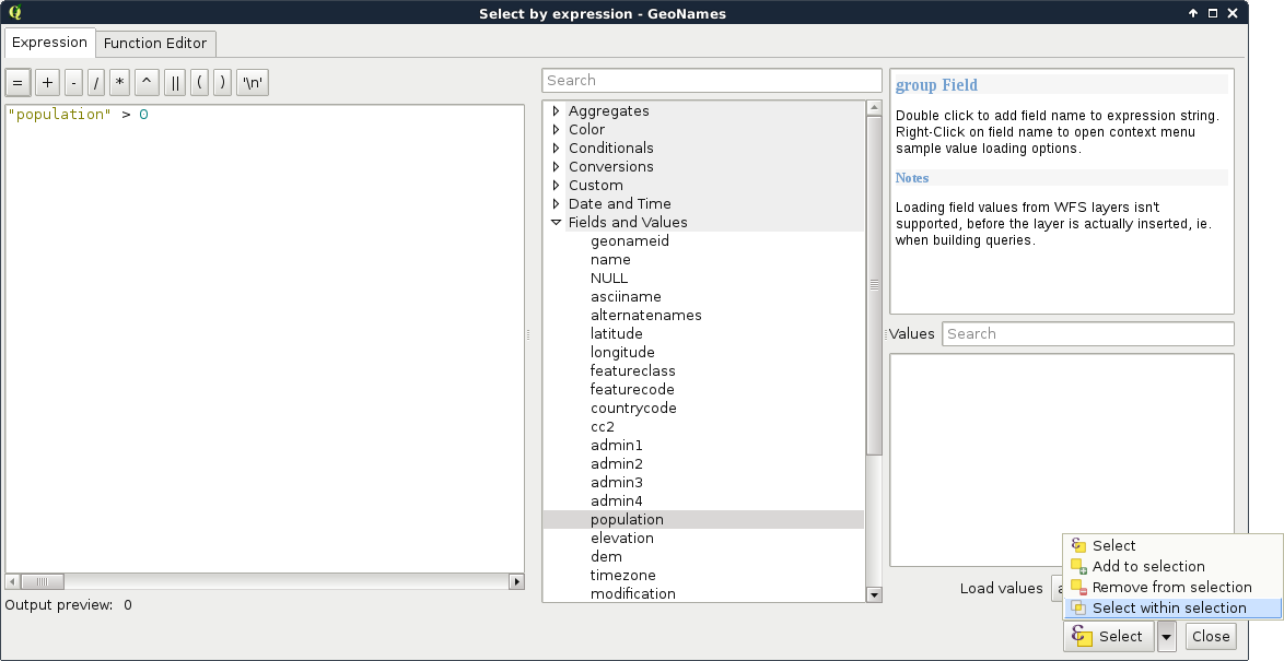
Lovely! The only problem, which I forgot to mention, is that we are only interested in features with a population value. The naive way to resolve this issue is to remove the selection, apply a filter on the GeoNames layer, and run the Select by location algorithm again. We can do better than that. If we open the query builder dialog, we can see some additional options next to Select by clicking on the arrow icon. We can add to the current selection, remove from it, and even select within the selection. For me, that is the most intuitive solution for this case. We just have to come up with a basic query and click on Select within selection:

    "population" > 0