Let's select the modified GeoNames layer and open the Select features using an expression tool. We can see QGIS's expression builder, which offers a very convenient GUI with a lot of functions in the middle panel, and a small and handy description for the selected function in the left panel. We do not even have to type anything to use some of the basic queries as QGIS lists every field we can access under the Fields and Values menu. Furthermore, QGIS can also list all the unique values or just a small sample from a column by selecting it and pressing the appropriate button in the left panel:

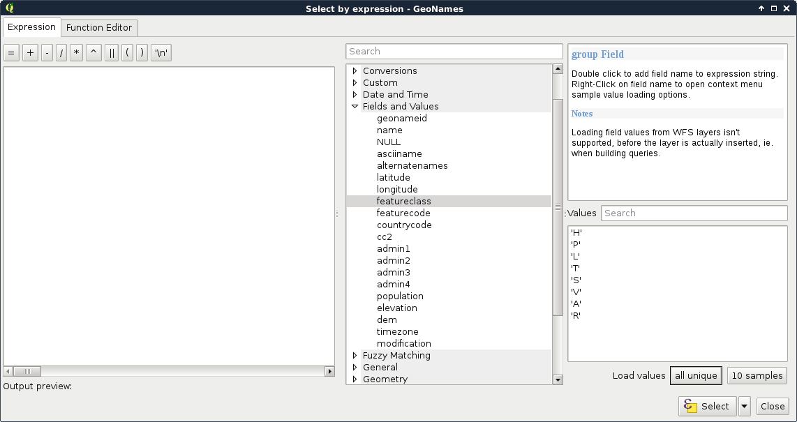
The basic SQL expressions that we can use are listed under the Operators menu. There, every operator is a valid PostgreSQL operator, most of them are commonly found in various GIS software. Let's start with some numeric comparisons. For that, we have to choose a numeric column. We can use the attribute table for that.

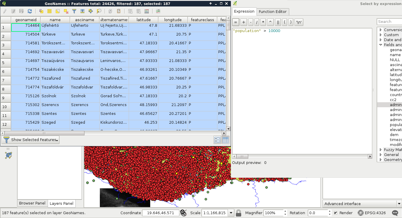
For basic numeric comparisons, let's choose the population column. In this first query, we would like to select every place where the population exceeds 10000 people. To get the result, we have to supply the following query:

    "population" > 10000

We can now see the resulting features as on the following screenshot:

If we would like to invert the query, we have an easy task, which is as follows:

    "population" <= 10000

We could do this as population is a graduated value. It changes from place to place. But what happens when we work with categories represented as numbers? In this next query, we select every place belonging to the same administrative area. Let's choose an existing number in the admin1 column, and select them:

    "admin1" = 10

The corresponding features are now selected on the map canvas:

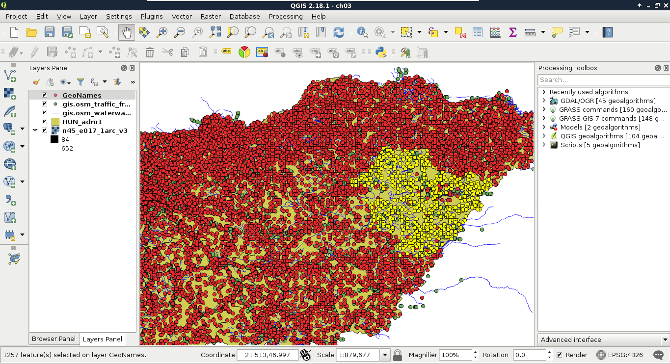
The canvas in the preceding screenshot looks beautiful! But how can we invert this query? If you know about programming, then you must be thinking about linking two queries logically together. It would be a correct solution; however, we can use a specific operator for these kinds of tasks, which is as follows:

    "admin1" <> 10

The <> operator selects everything which is not equal to the supplied value. The next attribute type that we should be able to handle is string. With strings, we usually use two kinds of operations--equality checking and pattern matching. According to the GeoNames readme, the featurecode column contains type categories in the character format. Let's choose every point representing the first administrative division (ADM1), as follows:

    "featurecode" = 'ADM1'

Of course, the inverse of this query is exactly the same like in the previous query (<> operator).

As the next task, we would like to select every feature which represents some kind of administrative division. We don't know how many divisions are there in our layer and we wouldn't like to find out manually. What we know from http://www.geonames.org/export/codes.html is that every feature representing a non-historic administrative boundary is coded with ADM followed by a number. In our case, pattern matching comes to the rescue. We can formulate the query as follows:

    "featurecode" LIKE 'ADM_'

In pattern matching, we use the LIKE operator instead of checking for equality, telling the query processor that we supplied a pattern as a value. In the pattern, we used the wildcard _, which represents exactly one character. Inverting this query is also irregular as we can negate LIKE with the NOT operator, as follows:

    "featurecode" NOT LIKE 'ADM_'

Now let's expand this query to historical divisions. As we can see among the GeoNames codes, we could use two underscores. However, there is an even shorter solution--the % wildcard. It represents any number of characters. That is, it returns true for zero, one, two, or two billion characters if they fit into the pattern:

    "featurecode" LIKE 'ADM%'

A better example would be to search among the alternate names column. There are a lot of names for every feature in a lot of languages. In the following query, I'm searching for a city named Pécs, which is called Pecs in English:

    "alternatenames" LIKE '%Pecs%'

The preceding query returns the feature representing this city along with 11 other features, as there are more places containing its name (for example, neighboring settlements). As I know it is called Fünfkirchen in German, I can narrow down the search with the AND logical operator like this:

    "alternatenames" LIKE '%Pecs%' AND "alternatenames" LIKE
     '%Fünfkirchen%'

The two substrings can be anywhere in the alternate names column, but only those features get selected whose record contains both of the names. With this query, only one result remains--Pécs. We can use two logical operators to interlink different queries. With the AND operator, we look for the intersection of the two queries, while with the OR operator, we look for their union. If we would like to list counties with a population higher than 500000, we can run the following query:

    "featurecode" = 'ADM1' AND "population" > 500000

On the other hand, if we would like to list every county along with every place with a population higher than 500000, we have to run the following query:

    "featurecode" = 'ADM1' OR "population" > 500000

The last thing we should learn is how to handle null values. Nulls are special values, which are only present in a table if there is a missing value. It is not the same as 0, or an empty string. We can check for null values with the IS operator. If we would like to select every feature with a missing admin1 value, we can run the following query:

    "admin1" IS NULL

Inverting this query is similar to pattern matching; we can negate IS with the NOT operator as follows:

    "admin1" IS NOT NULL