While superfluous columns are often present in general data, it is not rare if we don't have the required attributes we would like to work with. If we are lucky, we can generate them based on other existing attributes, although we should not worry if this is not the case. If we can prepare a table which can be joined to the existing one on a matching column, we can easily join them together.

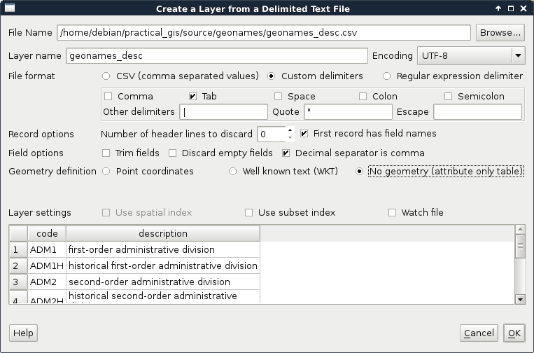
For this example, I prepared a small table containing descriptions of our GeoNames layer's featureclass and featurecodes columns based on the official GeoNames code page mentioned before. It is called geonames_desc.csv and you an access it from the supplementary material's ch03 folder or download it directly from https://gaborfarkas.github.io/practical_gis/ch03/geonames_desc.csv. The formatting of this table resembles the original GeoNames table as it is tab separated; however, it does not have any geometries. It only contains two columns--a code and a description. Let's open the table with the Add Delimited Text Layer tool. The first line is the header and the separator is the tab character. As we have no geometries, we should also state that by checking the No geometry option:

When the table is opened, we can see its entry in the Layers Panel. It has a special icon as it only consist of attributes. Now we can join the two layers. To start a join, we have to open the Properties of the target layer, in our case, GeoNames. There is a tab named Joins, which offers tools for managing different joins. These kinds of attribute joins do not result in overwriting the target layer, they are handled in memory; therefore, we can dynamically change them (add new ones, modify, and remove existing ones).

A successful join in QGIS needs some conditions to be met. We need a common column in both the tables as keys. These key columns hold the join conditions. The join procedure pairs these key columns together and joins the other columns of the joined layer accordingly. Therefore, to avoid ambiguities, we should have a target key column without null values and a joined key column with unique values. The key column of the joined table is never included in a join as it would introduce unnecessary redundancy. We can define a join the following way:

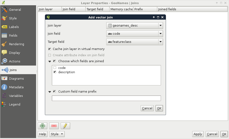
1. Access the Add vector join dialog with the green plus icon.
2. Fill the Join layer parameter, which is the layer or table we would like to join. In our case, it is the recent geonames_desc table.
3. Fill the Join field parameter, which is the key column of the joined layer. In our case, it is the code column.
4. Fill the Target field parameter, which is the key column of the target layer. In our case, it is the featureclass column.

We can also select the columns that we would like to join from the target table. As we have only two columns and one of them is the key column, we don't have to limit them. There is one final option for the prefix. As we can have an arbitrary number of joins and different tables can have the same column names, QGIS offers us the ability to prefix the target table's column names with the table's name. We can safely remove the prefix as we won't have further joins. To confirm the join, we have to click on OK not only in the dialog but also in the Properties window as simply closing it is the same as clicking on Cancel:

If we open the attribute table of our GeoNames layer, we can see the new description column appended. Furthermore, if we open the query builder, select the featureclass field, and query all the unique values, and do the same for the description field, we can see the number of unique values that match. Now let's edit the join in the Properties window. We can do that by selecting the join entry and clicking on the pencil icon. For the Target field, let's select the featurecode column. By inspecting the attribute table again, we can see that the values have changed and represent the description of the feature codes.

Attribute-based joins in QGIS work like left outer joins in SQL. QGIS takes every row from the target layer and matches a row from the joined table if it can. If there is no matching value, it fills the row with a null value. Every excess field is dropped from the joined table. For example, our description table contains descriptions for both feature classes and feature codes. Based on the key columns, one set of them is joined while the other is dropped.