
We already used some techniques to speed up queries, although we have a lot more possibilities in tuning queries for faster results. To get the most out of our database, let's see how queries work. First of all, in RDBMS jargon, tables, views, and other similar data structures are called relations. Relation data is stored in files consisting of static-sized blocks (pages). In PostgreSQL, each page takes 8 KB of disk space by default. These pages contain rows (also called tuples). A page can hold multiple tuples, but a tuple cannot span multiple pages. These tuples can be stored quite randomly through different pages; therefore, PostgreSQL has to scan through every page if we do not optimize the given relation. One of the optimization methods is using indexes on columns just like the geometry columns, other data types can be also indexed using the appropriate data structure.
There is another optimization method which can speed up sequential scans. We can sort our records based on an index we already have on the table. That is, if we have queries that need to select rows sequentially (for example, filtering based on a value), we can optimize these by using a column index to pre-sort the table data on disk. This causes matching rows to be stored in adjacent pages, thereby reducing the amount of reading from the disk. We can sort our waterways table with the following expression:
CLUSTER spatial.waterways USING sidx_waterways_geom;
In this preceding query, the sidx_waterways_geom value is the spatial index's name, which was automatically created by QGIS when we created the table. Of course, we can sort our tables using any index we create.
For the next set of tuning tips, we should understand how an SQL expression is turned into a query. In PostgreSQL, there are the following four main steps from an SQL query to the returned data:
- Parsing: First, PostgreSQL parses the SQL expression we provided, and converts it to a series of C structures.
- Optimizing: PostgreSQL analyzes our query, and rewrites it to a more efficient form if it can. It strives to obtain the least complex structure doing the same thing.
- Planning: PostgreSQL creates a plan from the previous structure. The plan is a sequence of steps required for achieving our query with estimated costs and execution times.
- Execution: Finally, PostgreSQL executes the plan, and returns the results.
For us, the most important part is planning. PostgreSQL has a lot of predefined ways to plan a query. As it strives for the best performance, it estimates the required time for a step, and chooses a sequence of steps with the least cost. But how can it estimate the cost of a step? It builds internal statistics on every column of every table, and uses them in sophisticated algorithms to estimate costs. We can see those statistics by looking at the PostgreSQL catalog's (pg_catalog) pg_stats view:
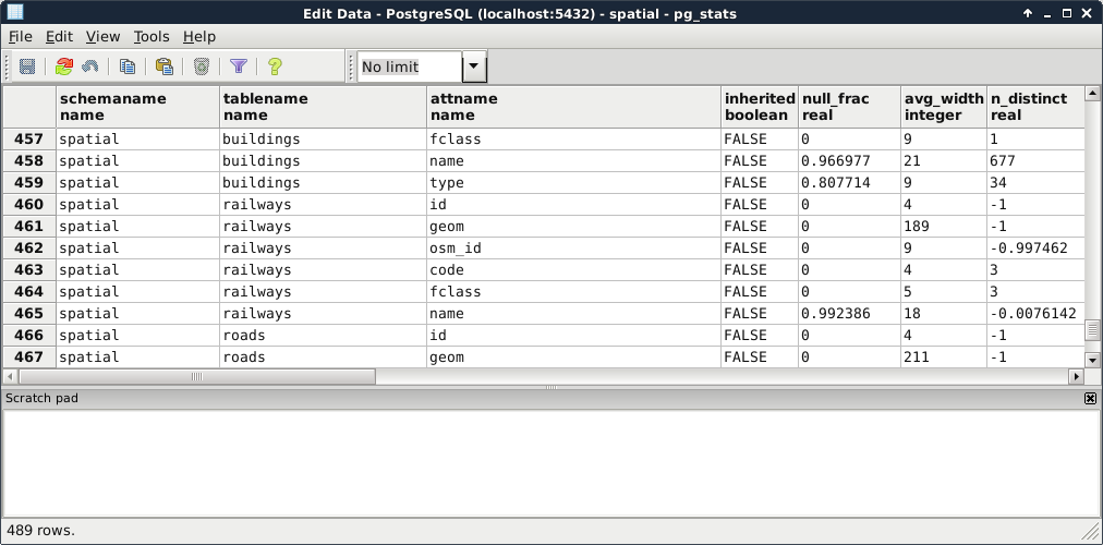
As the planner uses these precalculated statistics, it is very important to keep them up to date. While we don't modify a table, the statistics won't change. However on frequently changed tables, it is recommended not to wait on the automatic recalculations, and update the statistics manually. This update usually involves a clean-up, which we can do on our waterways_curve table by running the following expression:
VACUUM ANALYZE spatial.waterways_curve;
PostgreSQL does not remove the deleted rows from the disk immediately. Therefore, if we would like to free some space when we have some deleted rows, we can do it by vacuuming the table with the VACUUM statement. It also accepts the ANALYZE expression, which recalculates statistics on the table. Of course, we can use VACUUM without ANALYZE to only free up space, or ANALYZE without VACUUM to only recalculate statistics. It is just a good practice to run a complete maintenance by using them both.
Now that we know how important it is to have correct statistics, and how we can calculate them, we can move on to real query tuning. Analyzing the plan that PostgreSQL creates involves the most technical knowledge and experience. We should be able to identify the slow parts in the plan, and replace them with more optimal steps by altering the query. One of the most powerful tools of PostgreSQL writes the query plan to standard output. From the plan structured in a human readable form, we can start our analysis. We can invoke this tool by prefixing the query with EXPLAIN. This statement also accepts the ANALYZE expression, although it does not create any kind of statistics. It simply runs the query and puts out the real cost, which we can compare to the estimated cost. Remember that inefficient query from the last chapter? Let's turn it into a query plan like this:
    EXPLAIN ANALYZE SELECT p.* FROM spatial.pois p,
     spatial.landuse l WHERE ST_Intersects(p.geom,
     (SELECT l.geom WHERE l.fclass = 'forest'));
We can see the query plan generated as in the following screenshot:
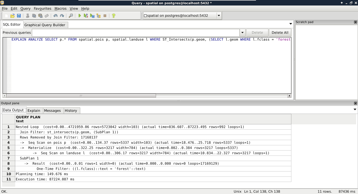
According to the query plan, in my case, we had to chew ourselves through about 5,700,000 rows. One of the problems is that this query cannot use indices, therefore, it has to read a lot of things into memory. The bigger problem is that it had to process more than 17 million rows, much more than estimated in the query plan. As PostGIS does spatial joins in such queries, and we provided a subquery as one of the arguments, PostGIS did a cross join creating every possible combination from the two tables. When I checked the row numbers in the tables, the POI table had 5,337 rows, while the land use table had 3,217 rows. If we multiply the two numbers, we get a value of 17,169,129. If we subtract the 17,168,137 rows removed by the join filter according to the executed query plan, we get the 992 relevant features. The result is correct, but we took the long way. Let's see what happens if we pull out our subquery into a virtual table, and use it in our main query:
    EXPLAIN ANALYZE WITH forest AS (SELECT geom
     FROM spatial.landuse l WHERE l.fclass = 'forest')
     SELECT p.* FROM spatial.pois p, forest f
     WHERE ST_Intersects(p.geom, f.geom);
By using WITH, we pulled out the geometries of forests into a CTE (Common Table Expression) table called forest. With this method, PostgreSQL was able to use the spatial index on the POI table, and executed the final join and filtering on a significantly smaller number of rows in significantly less time. Finally, let's see what happens when we check the plan for the final, simple query we crafted in the previous chapter:
    EXPLAIN ANALYZE SELECT p.* FROM spatial.pois p,
     spatial.landuse l
     WHERE ST_Intersects(p.geom, l.geom)
     AND l.fclass = 'forest';
The query simply filters down the features accordingly, and returns the results in a similar time. What is the lesson? We shouldn't overthink when we can express our needs with simple queries. PostgreSQL is smart enough to optimize our query and create the fastest plan.
There are some scenarios where we just cannot help PostgreSQL to create fast results. The operations we require have such a complexity that neither we, nor PostgreSQL, can optimize it. In such cases, we can modify the memory available to PostgreSQL, and speed up data processing by allowing it to store data in memory instead of writing on the disk and reading out again when needed. To modify the available memory, we have to modify the work_mem variable. Let's see the available memory with the following query:
SHOW work_mem;
The 4 MB RAM space seems a little low. However, if we see it from a real database perspective, it is completely reasonable. Databases are built for storing and distributing data over a network. In a usual database, there are numerous people connecting to the database, querying it, and some of them are also modifying it. The work_mem variable specifies how much RAM a single connection can take up. If we operate a small server with 20 GB of RAM, let's say we have 18 GB available for connections. That means, with the default 4 MB value, we can have less than 5,000 connections. For a medium-sized company operating a dynamic website from that database, allowing 5,000 people to browse its site concurrently might be even worse than optimal.
On the other hand, having a private network with a spatial database is a completely different scenario. Spatial queries are usually more complex than regular database operations, and complex analysis in PostGIS can take up a lot more memory. Let's say we have 20 people working in our private network using the same database on the same small server. In this case, we can let them have a little less than 1 GB of memory for their work. If we use the same server for other purposes, like other data processing tasks, or as an NFS (Network File System), we can still give our employees 128 MB of memory for their PostGIS related work. That is 32 times more than they would have by default, and only takes roughly 2 GB of RAM from our server.
In modern versions of PostgreSQL, we don't have to fiddle with configuration files located somewhere on our disk to change the system variables. We just have to connect to our database with a superuser role, use a convenient query to alter the configuration file, and another one for reloading it and applying the changes. To change the available memory to 128 MB, we can write the following query:
ALTER SYSTEM SET work_mem = '128MB';
Finally, to apply the changes, we can reload the configuration file with this query:
SELECT pg_reload_conf();