Congratulations on your first analysis! It was quite an adventure, right? What we've done is more than mere spatial analysis. We conceptualized a model, and made an analysis according to that. Our model stated that the vicinity of the requested amenities and features can be translated to 500 meters. Quiet places are places which are more than 200 meters away from busy roads, and more than 500 meters away from industrial places. Are these numbers exact? Of course not. They are approximations of real-world phenomena, and therefore, models.

What happens if one of the customers says that our analysis is faulty? Some of the results are too close to noisy places, others are too far from markets. We can try some other distances to make our model satisfy the customer better, although we would need to run the entire analysis every time. Luckily, in modern desktop GIS software like QGIS, there is a graphical modeler to create, save, and modify a step-by-step analysis by connecting algorithms to each other. It is like a block-based programming language for analysts. We can link existing algorithms (even models) together to create a graphical process model, that QGIS then interprets and executes.

We can access QGIS's graphical modeler from the menu bar via Processing | Graphical Modeler. First of all, we need to name our model, and categorize it in a group. I used the name House search and the group Vector. If we save a new model, we have to specify a file name, which can be anything as long as we don't change the default directory QGIS offers, and use a unique file name. If we close the model, we can see it under the category we specified. We can edit our existing models by right-clicking on them, and selecting Edit model:

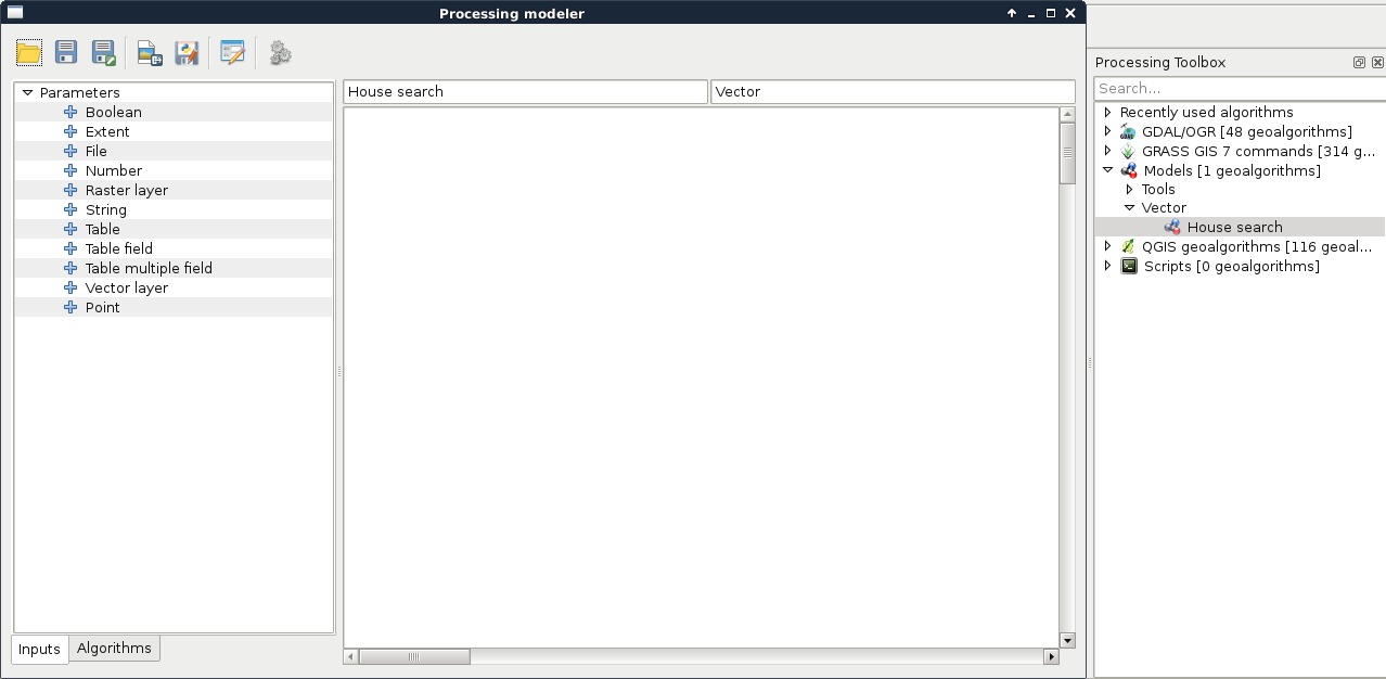
The graphical modeler has a lot of capabilities from which we will only use the most necessary ones to create our model. The left panel shows the inputs and algorithms we can use. We can simply drag and drop the needed blocks to the right panel, which is the canvas of our model. As the first step, let's create the quiet homes part. For this, we need three input vector layers--a point layer for the Houses, a line layer for the Roads, and a polygon layer for Land use. When we drop a Vector layer input to the canvas, we can specify the name and the type of the input layer:

Now, if we save our model, and run it with the Run model button or by opening it from the processing toolbox, we can see our three constrained input vector layers just like in any other QGIS algorithm. Now we need to drag and drop some algorithms from the Algorithms tab of the left panel, which will use our input layers:

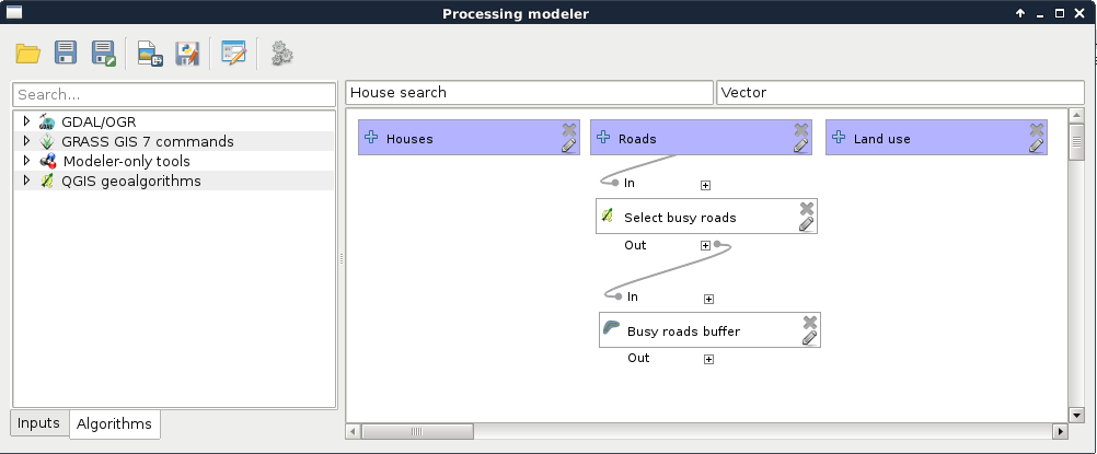
1. Drag in the first algorithm--QGIS geoalgorithms | Vector selection tools | Select by expression. Select the Roads layer as an input layer, and provide the expression "fclass" LIKE 'motorway%' OR "fclass" LIKE 'primary%'. Give it the description Select busy roads.
2. Drag in a Fixed distance buffer algorithm. Select the output of the previous tool as an input, and define a buffer zone of 200 meters. You can also dissolve the result. Give it a description, something like Busy roads buffer:

As we can see, we have access to some extra features besides the regular parameters that QGIS offers in the graphical modeler. These include the following:

• Description: We can describe an algorithm, as the graphical modeler can hold multiple instances of the same tool. This way, we can distinguish between them when we build the rest of our model. Always add a unique description.
• Parameters: These are the regular parameters that QGIS requires.
• Output: Some of the algorithms can produce an output. If we give it a name, QGIS treats it as a result, and offers us to save it somewhere. If not, QGIS knows that it is just an intermediary step producing temporal data.
• Parent algorithms: We can affect the order of execution by setting additional parent algorithms of a geoalgorithm.

Let's finish modeling the first step of our analysis with the following steps:

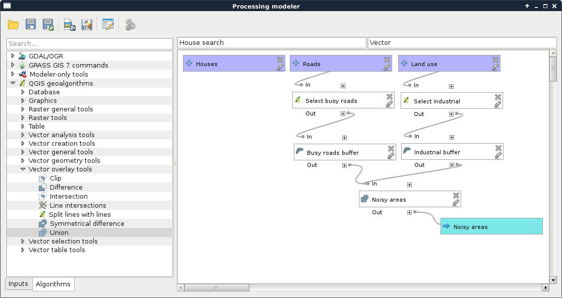
1. Add another Select by expression tool. The input should be the Land use layer this time, while the expression is "fclass" = 'industrial' OR "fclass" = 'quarry'.
2. Add another Fixed distance buffer tool. The input should be the selected land use layer, and the buffer distance should be 500 meters. You can dissolve the result.
3. Add a Union tool. The two inputs should be the two buffered layers. Specify an output name, as we can test our model that way.
4. Save the model, and run it:

Now we can see something, which highly resembles the geoalgorithms we are used to in QGIS. It requires three inputs, and gives one output. Let's remove the filters from the required layers, specify them as input parameters, and run the query.

By running the model, we can notice a few things. First of all, the result is similar to the unified buffer zones we created step by step. However, we can do the whole workflow by simply pressing a single button. However, the model is seemingly quite slow. More precisely, dissolving the buffers slows down the whole process. We can do these few things about that:

• We can disable dissolving, which will make buffering faster, but union slower.
• We can build a geometry index on the inputs of the buffers with QGIS geoalgorithms | Vector general tool | Create spatial index.
• We can save the selected features or use the Extract tools instead of the Select tools. QGIS models and PostGIS selections are not the greatest duo, especially when a spatial query follows, because they decrease performance.

For now, let's just finish the current part of the analysis:

1. Edit the model.
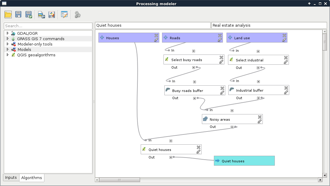
2. Remove the output produced by the Union tool. You just have to remove the text from the Union<OutputVector> field.
3. Add an Extract by location algorithm. We should select from the Houses layer, specify the unified buffers as the intersection layer, and intersects as the spatial predicate.
4. Specify an output to the Extract by location algorithm.
5. Rename the model to something like Quiet houses, and the group to Real estate analysis.
6. Save the model.

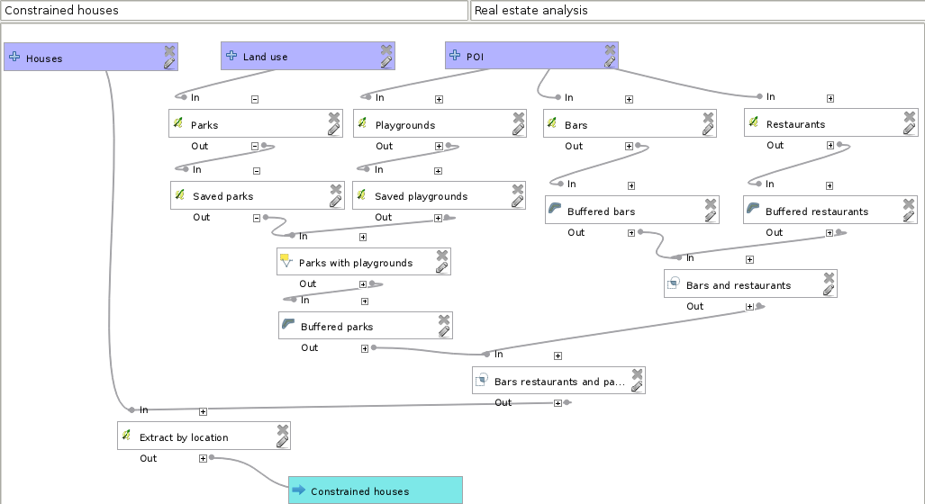
Now we have the Quiet houses produced by our model. The next part is to constrain those houses with the preferences of our customers. To keep our final model clean, we are going to separate different tasks. Let's create another model with a name like Constrained houses, and with the previous model's group name:

1. Add three input vector layers--one for the Houses, one for the Land use, and one for the POI layers.
2. Select the parks from the Land use layer, and the playgrounds from the POI layer. Save the selected features. As both the selections only take a single key and value, you can use a single Extract by attribute tool instead ("fclass" = 'park' from the Land use layer and "fclass" = 'playground' from the POI layer).
3. Select parks in the vicinity of playgrounds, and buffer the results.
4. Select bars from the POI layer, and buffer the results.
5. Select restaurants from the POI layer, and buffer the results.
6. Intersect the buffered layers. First take two of them as the input of an Intersection, and then take the result with the third buffered layer as inputs of another Intersection.

7. Extract houses located in the final result. Name the output of this final step:

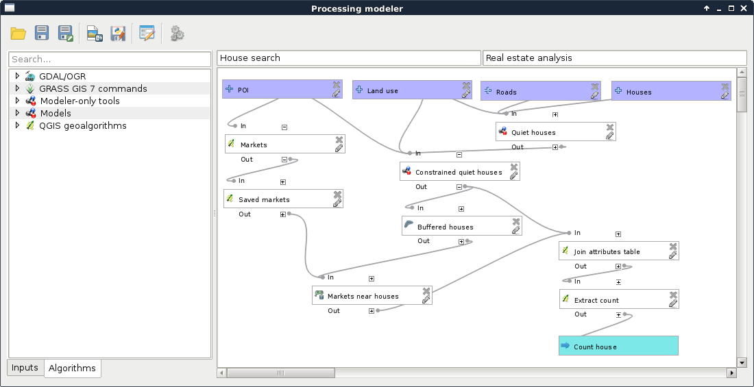
Our final model should contain every input, our other models, and the rest of the analysis:

1. Create a new model with a name something like House search or House analysis in the same group.
2. Create four inputs for the house, road, land use, and POI layers.
3. Add the Quiet houses model, and specify the inputs.
4. Add the Constrained houses model specifying the output of the previous model as the House layer input, and the rest of the input layers as the other inputs.
5. Buffer the result of the previous model.
6. Select the markets from the POI layer, and save the selection.
7. Use Count points in polygon to count the number of markets in the houses' buffer zones.
8. Join the output of the Constrained houses model with the result of the previous tool by using QGIS geoalgorithms | Vector general tools | Join attribute table. Both the table fields should be id.
9. Extract the valid features by using the expression count >= 2. We can use the Extract by attribute tool for this:

Let's test our model by running it and examining the results. If something really weird did not occur, we've got bad results. Not just slightly I must have done something wrong in my step-by-step workflow bad results, but really bad ones. Why did something like this happen? In a nutshell, QGIS does not have a concept about correct order. It interprets our model, and orders the algorithms based on inputs. Every algorithm has so many dependencies as inputs, which must be executed before them. Other algorithms are executed in an arbitrary order, which is good, as QGIS 3 will be able to run processing algorithms in parallel.

I'm sure you already found out the solution for this ordering problem--we must make sure that order does not matter. This can be achieved by chaining algorithms in a way that our steps do not rely on the state of the data. If we think it through, in our model, data has state only in a few cases; that is, when we use selections. We have the following two ways to resolve this problem:

• We can discard selections, and work with extraction algorithms where we can. Where we cannot, we can build an Extract by expression model (Appendix 1.8), and use that instead.
• We can force correct ordering by defining additional parent algorithms for some of our steps.

Let's stick with the second option now. If we think about the possible orders of execution in our models, we can conclude that the Quiet houses model is safe. No matter in which order QGIS executes it, we will always get the same results. On the other hand, there are several incorrect paths in the Constrained houses model, and an additional one in our final model. In the Constrained houses model, we select three times from the same POI layer. If the second selection (bars) occurs after the playgrounds are selected, but before they are saved, we get incorrect results. Let's correct it by defining the Saved playgrounds step as a prerequisite to the Bars step:

1. Edit the Constrained houses model.
2. Edit the Bars step with the pencil icon, or by right-clicking on it and selecting Edit.
3. Click on the chooser (...) button besides the Parent algorithms field.
4. Select the Buffered Parks algorithm. We do not have the unique names we gave to our steps in this dialog, although when we select an algorithm, QGIS connects the two steps together with a grey line. Check the result, and if the wrong algorithm got connected, try again.

Using the same procedure, we should make the Buffered bars step a prerequisite to the Restaurants step, as that is the second place where an error can occur. When done, let's inspect our final model. There we select the markets, and save them to another layer. However, what happens if our second model runs after the selection, but before the extraction? The correct selection is gone, and a wrong selection gets saved. To deal with this possibility, we have to make our Constrained quiet houses step a prerequisite to our Markets step. If we run our model again, the results should be the same as the ones gained from our step-by-step approach.