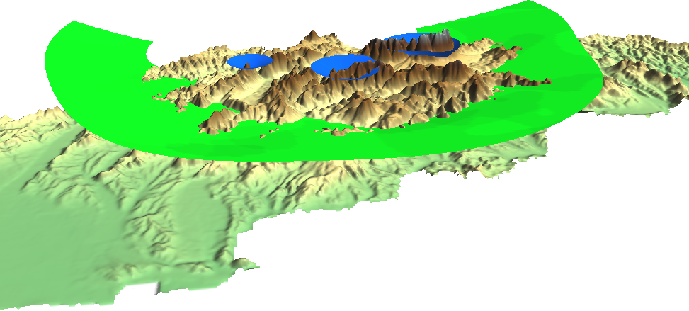
Appendix 1.1: Isosurfaces (800 mm and 1200 mm precipitation) visualized on the Digital Elevation Model of Slovakia provided by the sample slovakia3d dataset for GRASS GIS:

Appendix 1.2: The same map we created in Chapter 2, Accessing GIS Data With QGIS, only with a CRS using an Albers Conic projection (EPSG:102008). The map is not North-aligned; therefore, a north arrow was used with the North alignment parameter set to True north:

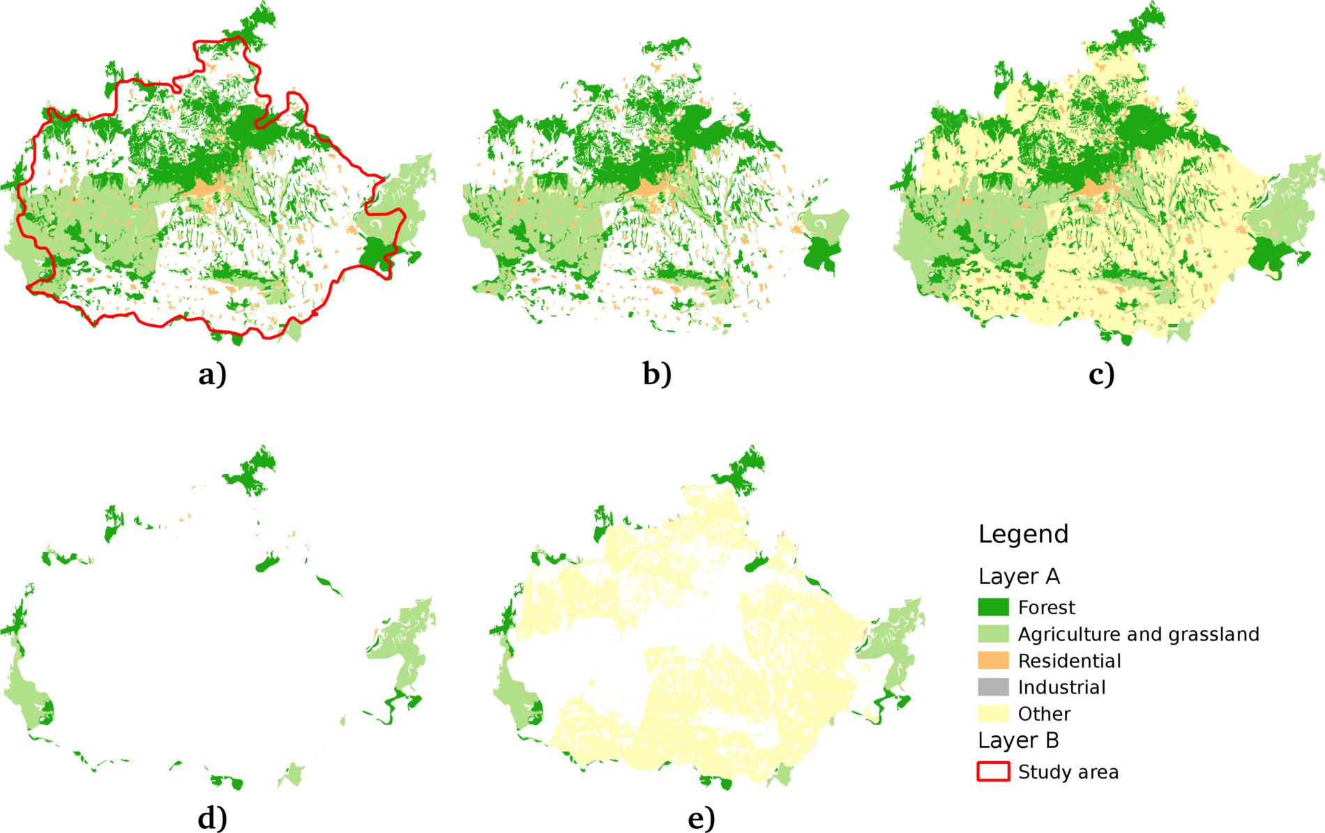
Appendix 1.3: Some of the basic geoalgorithms visualized. a: the two input layers (A and B per GRASS's v.overlay), b: clip (and), c: union (or), d: difference (nor), e: symmetrical difference (xor):

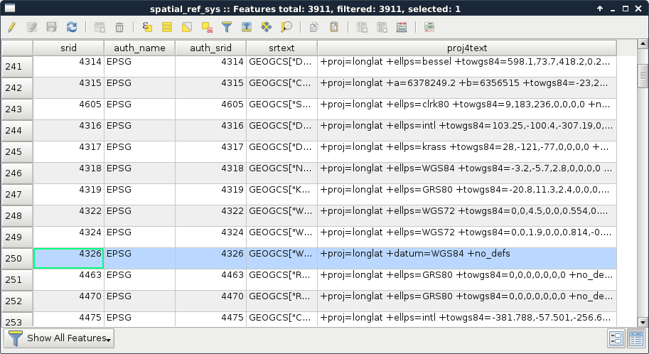
Appendix 1.4: Some of the Coordinate Reference System's PostGIS support. The selected one is the EPSG:4326 CRS used by the book in the early chapters:

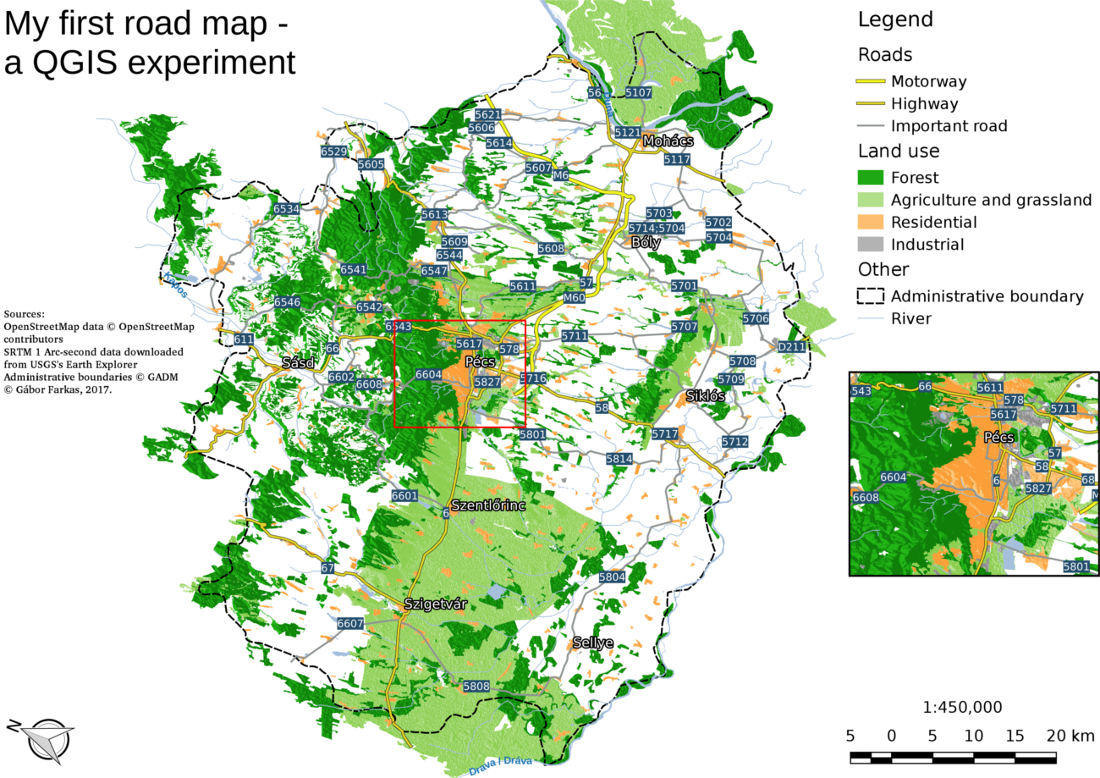
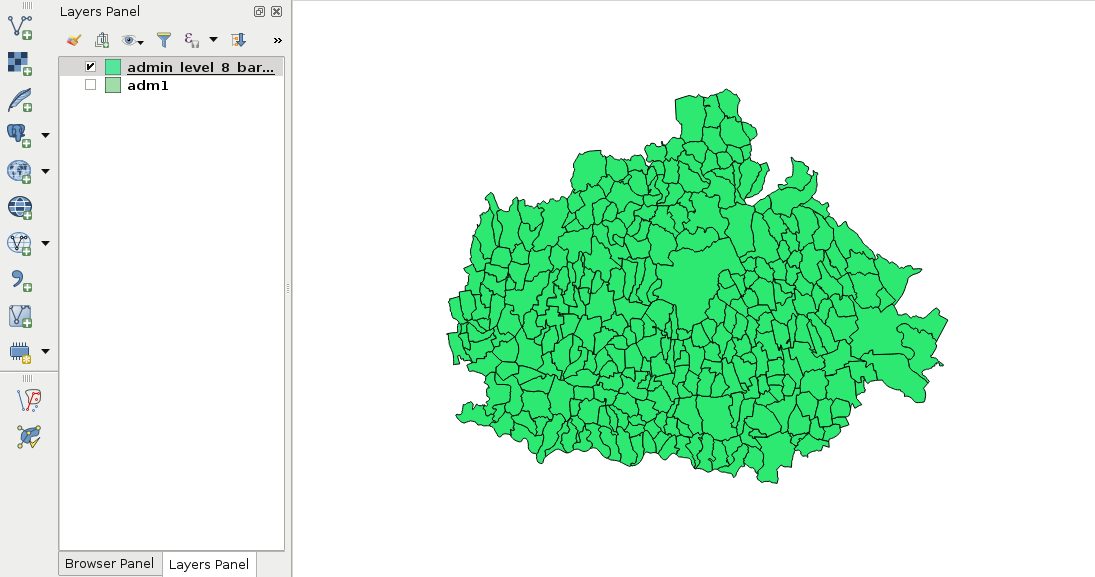
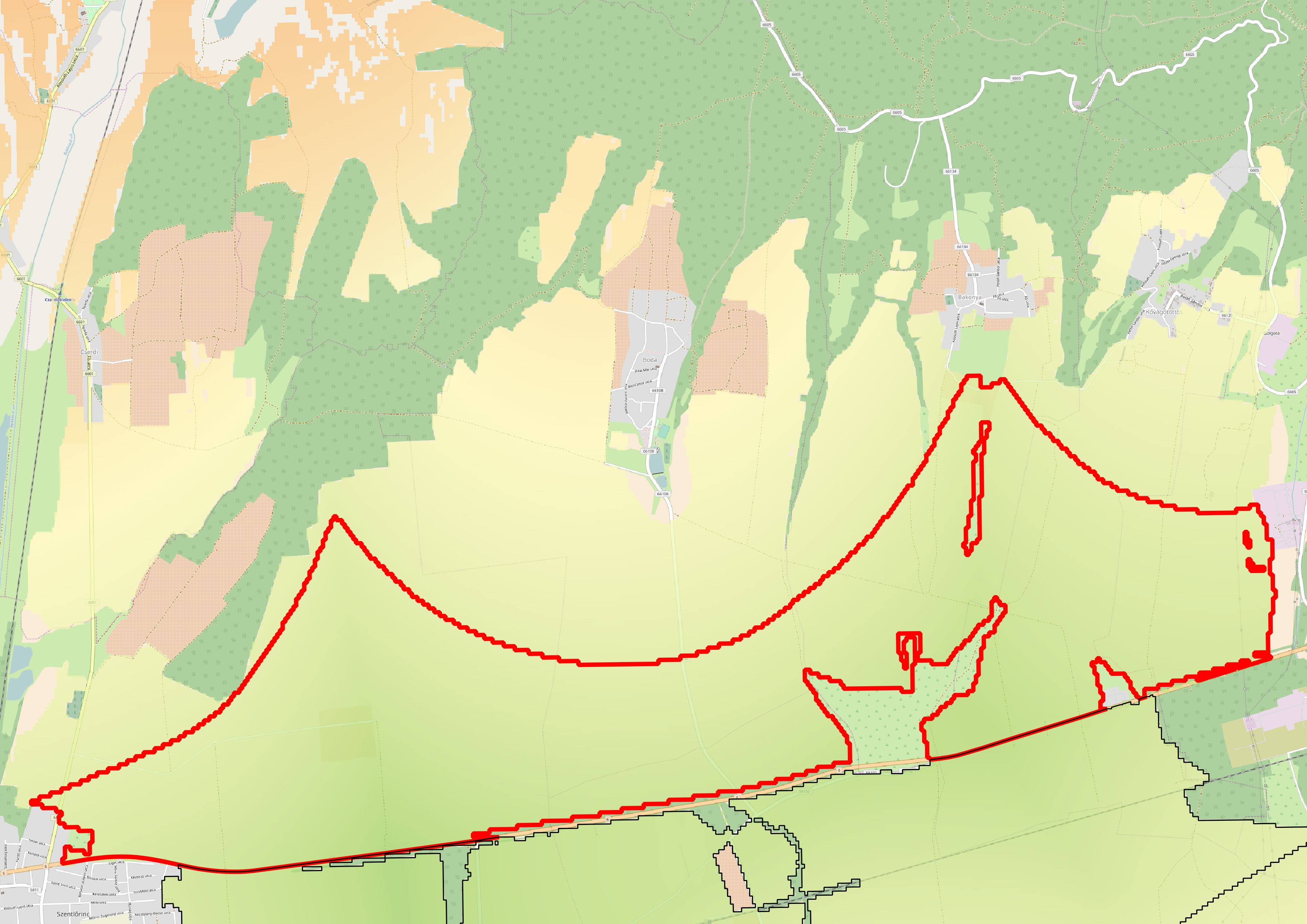
Appendix 1.5: Settlement data of my study area downloaded from the OpenStreetMap database via the QuickOSM plugin using the Overpass API:

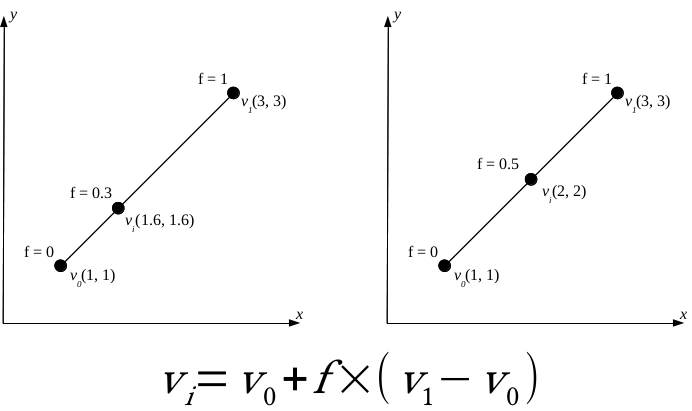
Appendix 1.6: Linear interpolation of point v_i on the line segment between points v₀ and v₁ based on a factor f. If v₁ - v₀ divided by 1/f leaves a remainder, the interpolated coordinate needs more precision (left). If not, the interpolated coordinate will have the same precision (right). In GIS, however, it is a common practice to store coordinates with a fixed precision in a single vector layer:

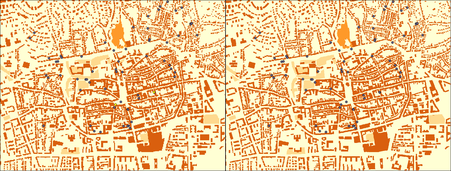
Appendix 1.7: Difference between precise proximity analysis with buffering (green points), and selecting features with precision values (yellow points) in QGIS. Every green point is selected, but there are some points excluded from the precise results:

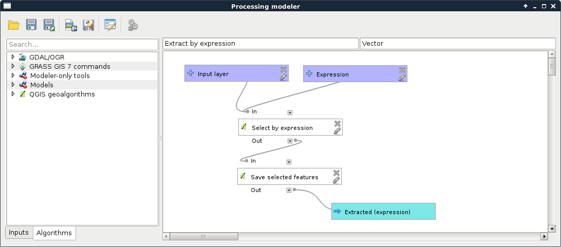
Appendix 1.8: Do you need an Extract by expression tool in QGIS? Build one yourself! You can easily create such a model by requiring a Vector layer input of any type, a String input for the expression, and linking the Select by expression and the Save selected features tools together:

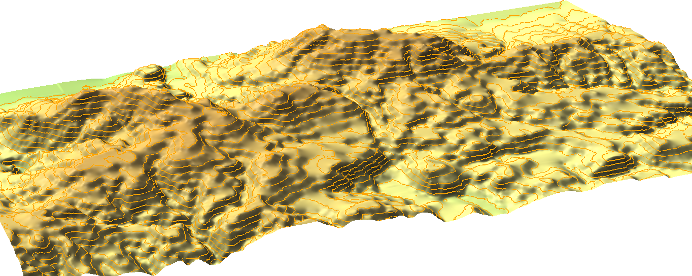
Appendix 1.9: Interpolated surface from contour lines visualized in 3D with the contour lines displayed on the interpolated surface:

Appendix 1.10: The same vector layer transformed to raster with a resolution of 5 meters (left) and 2 meters (right). By using 5 meters, two of the possible houses overlap with buildings; thus, get cut off roads in the walking time analysis:

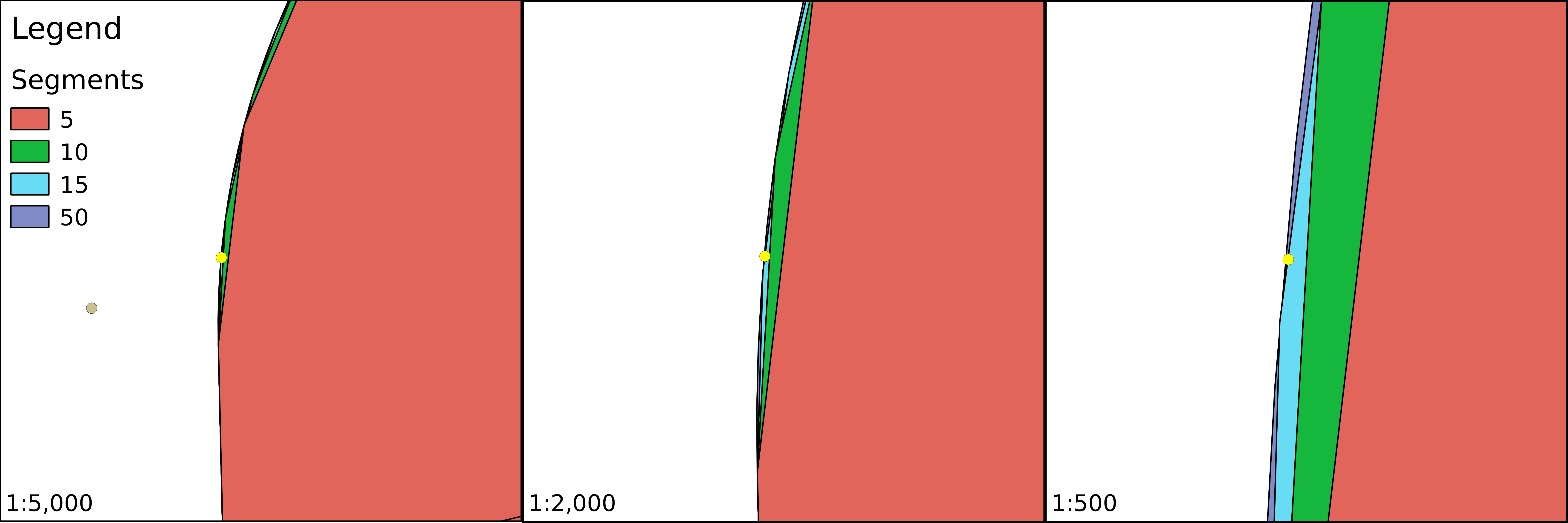
Appendix 1.11: Buffer zones with a different number of segments are used for more precise approximations. The yellow point lies outside of the buffer zones created with 5 and 10 segments; however, it is only a matter of precision as it is located inside the zones as proven by the buffers created with 15 and 50 segments:

Appendix 1.12: Three popular distance types in GIS. In the Manhattan distance (left), we can go only in one dimension at a time; in the euclidean distance (center), we can move in two dimensions at a time; while in the case of the great-circle distance (right), we can move in three dimensions at a time, but only on the surface of a sphere. Note that the Manhattan distance between the same pair of points does not change, no matter how many breaks (turns) we use:

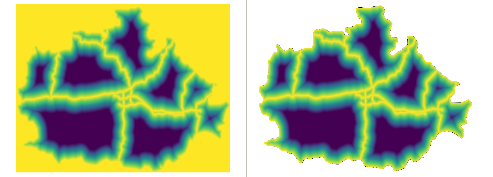
Appendix 1.13: Using clipped layers with NoData values in GDAL's Proximity tool introducing edge effects (left). NoData values are reclassified to zeroes, which wouldn't be a problem; however, distances are calculated from the edges, like they were features. It does not matter if we clip the distance matrix again (right), the edge effects are already introduced to the analysis:

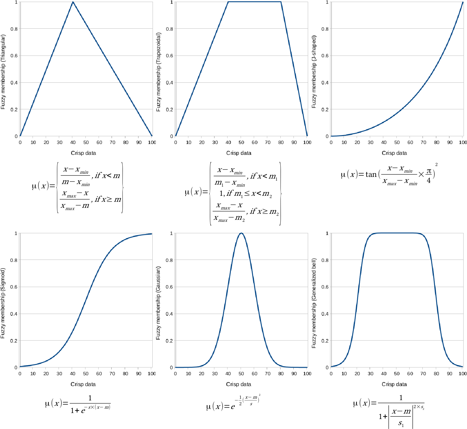
Appendix 1.14: Other popular fuzzy membership functions. Some of them are similar to the ones described in Chapter 10, A Typical GIS Problem, although with slightly different shapes and different formulas. The formulas were created with the assumption that the whole data range is fuzzified. If not, cell values below or above the threshold should be handled. In the formulas, variables denoted with m are break points or turning points, while variables denoted with s are defining the shape of the functions.

The natural number e is not included in QGIS's raster calculator, although, similarly to π, it can be hard coded as 2.7182:

Appendix 1.15: Using an OpenStreetMap base layer under the suitability map. The suitability map has a transparency of 30%:

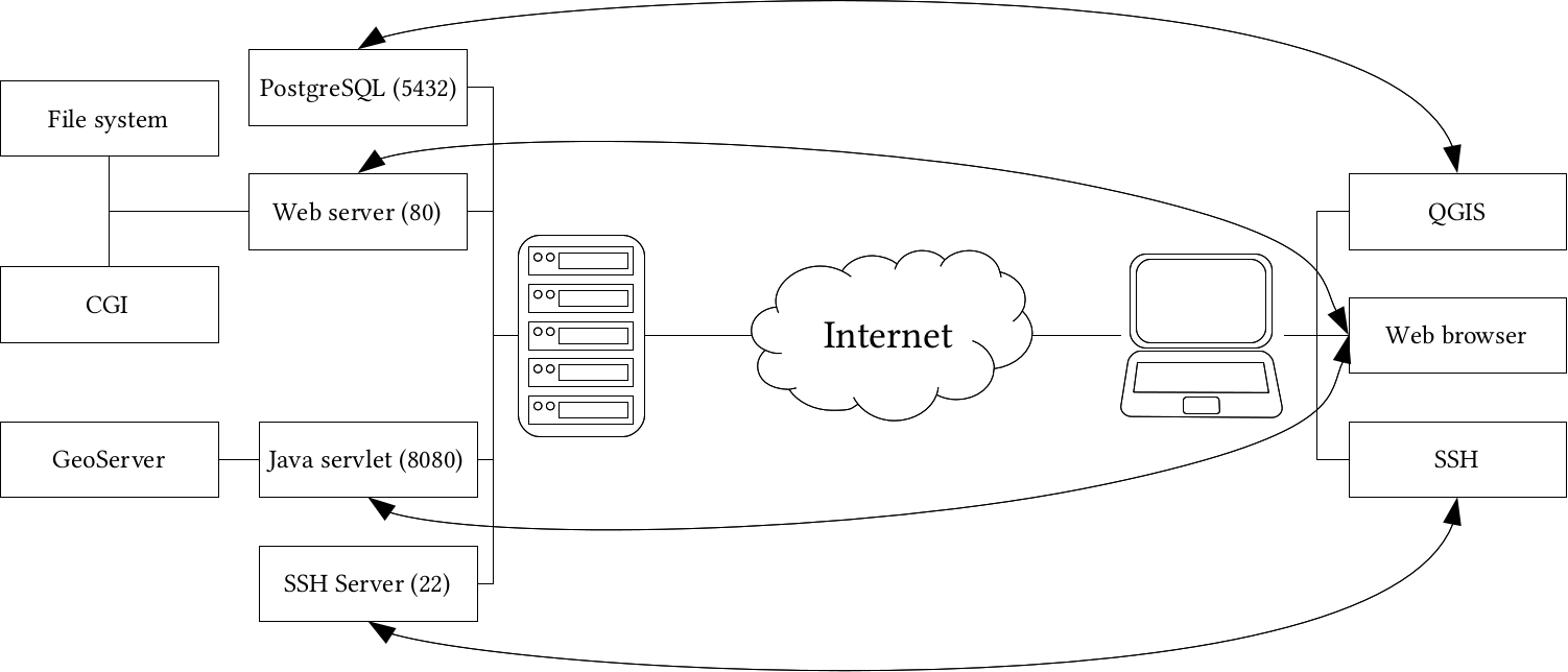
Appendix 1.16: A server machine hosting two web servers (one for running Java web applications), a PostgreSQL database, and an SSH server. Clients can query those servers with the appropriate client-side applications:

Appendix 1.17: Hillshaded land uses polygons in GeoServer. You can achieve the same by using Raster | Analysis | DEM in QGIS with the default Hillshade mode to create a static relief raster. Then, you can clip the relief to the area of the polygons using Raster | Extraction | Clipper with the option of cropping the result to the cutline. Finally, you have to load the resulting raster into GeoServer, and blend it into the land use layer using an overlay composition:

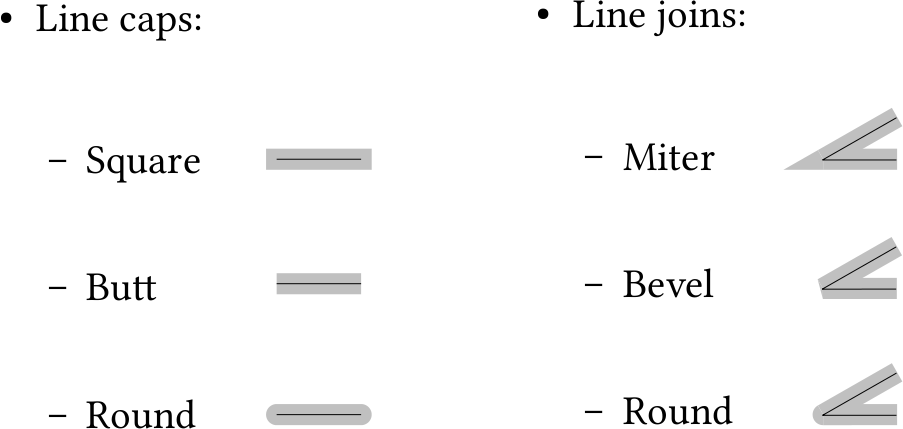
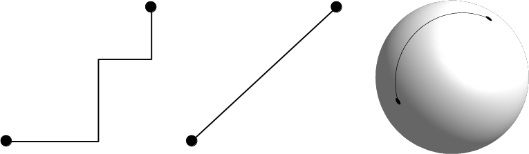
Appendix 1.18: Common line cap and line join styles used in vector graphic software: