
Next, let's create some complex styling to visualize our main roads similar to the visualization we created in QGIS:
- Create a new style. Name it accordingly, and limit it to our workspace.
- Select the CSS option in the Format field.
- Generate a line template, save the style, reopen it, and preview it on our roads layer.
- Rewrite the rule as follows to show secondary roads, as they had a simple symbolizer:
        /* @title Important roads */
        [fclass LIKE 'secondary%'] {
         stroke: #8f9593;
         stroke-width: 1;
        }
- It's time to create the complex line styles. In SLD, we would have to create multiple <FeatureTypeStyle> elements to have multiple lines drawn on each other. In CSS, however, we can define multiple styles in a single definition separated by commas. Similarly, we can define their other attributes the same way. The order of the values is the only thing what matters:
        /* @title Motorways */
        [fclass LIKE 'motorway%'] {
         stroke: #000000, #eff21e;
         stroke-width: 4, 3;
        }
        /* @title Highways */
        [fclass LIKE 'primary%'] {
         stroke: #000000, #ded228;
         stroke-width: 3, 2;
        }
Note that in QGIS, we defined line widths in millimeters. In GeoServer, we usually define widths in pixels. Therefore, you might need to fiddle with the width values a little bit to get aesthetic results.
Our complex line styles should look like the following:
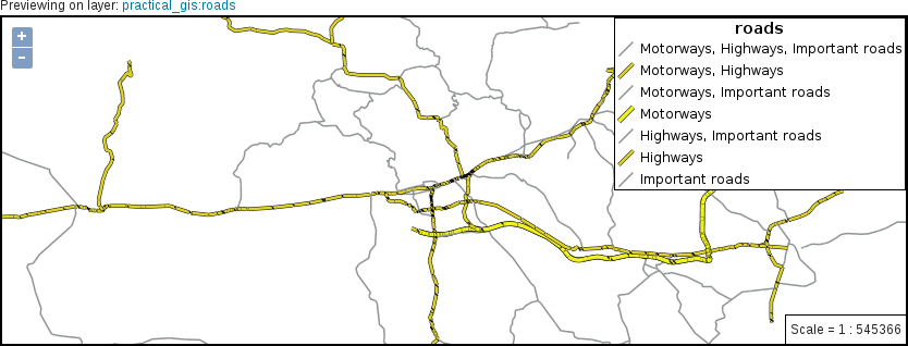
- We've got some better results, although our map still suffers from the symbol levels problem like in QGIS. In GeoServer, for altering the order of rendering lines with different styles, we can use the z-index property. When we have multiple styles assigned to a single-line type, we have to use multiple z-indices separated by commas. Before applying the symbol levels, find out the correct order. The black borders should come first, while the rest of the roads should be drawn according their priorities. Important roads second, highways third, and motorways, fourth:
        /* @title Motorways */
        [fclass LIKE 'motorway%'] {
         stroke: #000000, #eff21e;
         stroke-width: 4, 3;
         z-index: 1, 4;
        }
        /* @title Highways */
        [fclass LIKE 'primary%'] {
         stroke: #000000, #ded228;
         stroke-width: 3, 2;
         z-index: 1, 3;
        }
        /* @title Important roads */
        [fclass LIKE 'secondary%'] {
         stroke: #8f9593;
         stroke-width: 1;
         z-index: 2;
        }
You can see the available CSS properties in the official reference at http://docs.geoserver.org/latest/en/user/styling/css/properties.html.
Now we should be able to see clean lines rendered by GeoServer:
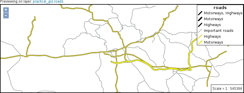
- The only problem left is the occasional gaps between our line segments. As GeoServer applies a butt line ending by default (Appendix 1.18), some of our segments get cut off in their meeting points. To solve this issue, we can round off all of our lines with a global definition as follows:
        * {
         stroke-linecap: round;
        }
It is a good practice to use clean, processed, visualization-ready vector data in GeoServer. Although GeoServer has some quite advanced capabilities to handle raw vector layers, it is far from a full-fledged GIS software.
- Finally, let's add some labels showing road references to important roads. If we add labels globally, we would end up with a map showing labels for every road no matter whether they are visualized or not. Therefore, we need a selector which selects only our features of interest. The labels should have a white color, and a bluish rectangular background. We can set a background with the shield property, which accepts a point symbolizer as a value. As we have a square symbol at hand, we can use that. When we put the code together, we should get something like the following:
        [fclass LIKE 'motorway%'], [fclass LIKE 'primary%'],
         [fclass LIKE 'secondary%'] {
          label: [ref];
          font-family: DejaVu Sans;
          font-fill: #ffffff;
          shield: symbol('square');
         }
- Although we have labels on our map, it still bleeds from several wounds. First of all, we need to offset our labels so that they are placed in the middle of our lines. We can achieve this by modifying the anchor point. The anchor point defines the reference point of our labels. It is placed in the middle of our lines, and the label is drawn from that point. By default, the anchor point is the lower-left point of our labels, which is represented with two 0s. As the upper-right coordinates are represented with two 1s, the middle point of our labels are two 0.5s:
label-anchor: 0.5 0.5;
- We should also remove duplicated labels. The default behavior of GeoServer is to render a label on every separate segment. As we have many segments, we get a lot of labels. Although there is no SLD option for merging logically coherent lines, GeoServer can do that with a vendor option. In CSS, we can also use vendor options prefixed with -gt-. The correct option for this is -gt-label-group, which renders a single label for lines with the same label attribute, on the longest segment:
-gt-label-group: true;
- Now we have fewer labels; however, regardless of their width, they are rendered on the same-sized square. We can override this behavior by using two vendor options---gt-shield-resize and -gt-shield-margin. The former defines how GeoServer should resize shields when the label sticks out, while the latter defines the margin size around the labels in pixels:
         -gt-shield-resize: stretch;
         -gt-shield-margin: 2;
- The only thing left to do is to customize the shields. Markers can be customized by using pseudo selectors to apply further properties to every symbol. In this case, we can safely customize every shield marker by using a sole :shield pseudo selector in a separate definition block, as we have only one type of shield.
        :shield {
         fill: #244e6d;
        }
Putting the whole code together, we get a label description similar to the following:
        [fclass LIKE 'motorway%'], [fclass LIKE 'primary%'],
         [fclass LIKE 'secondary%'] {
         label: [ref];
         font-family: DejaVu Sans;
         font-fill: #ffffff;
         label-anchor: 0.5 0.5;
         shield: symbol('square');
         -gt-label-group: true;
         -gt-shield-resize: stretch;
         -gt-shield-margin: 2;
        }
        :shield {
         fill: #244e6d;
        }
If you have multiple types of shields to style individually, you can nest the definition block of the shield pseudo element into the definition block of the labels using it. You can read more about nested rules at http://docs.geoserver.org/latest/en/user/styling/css/nested.html.
If we apply the final style as the default on the roads layer, and override the road layer's style of our layer group in Data | Layer Groups, we can see our final composition in Data | Layer Preview:
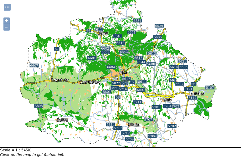
GeoServer cares less about label collisions than QGIS. To reduce overlapping labels, you can increase the minimum required space in pixels between adjacent ones with the -gt-label-padding vendor option.