The atlas generator is the most powerful feature of QGIS's print composer. It can create a lot of maps automatically based on a template we provide. The underlying concept is very basic--we have to provide a polygon layer with a column which has unique values. The print composer takes that layer, and creates a separate map page for every different value (therefore, feature) it can find in the provided column. Furthermore, it grants access to the current feature it uses for the given page. The real power comes from the QGIS expression builder, which enables us to set cartographic preferences automatically. With this, we can build a template for our atlas and use it to showcase each suitable area in its own map.

First of all, if we would like to create a front page with every suitable area on a single map, we have to create a feature enveloping the polygons from our suitable areas polygon layer. We can create such a polygon with QGIS geoalgorithms | Vector geometry tools | Convex hull. It takes a vector layer as an argument, and creates a single polygon containing the geometries of the input features:

1. Create the convex hull of the suitable areas using the aforementioned tool. Save the output to the working folder, as the merge tool does not like memory layers.
2. Open the attribute table of the convex hull layer. Remove every attribute column other than id. They would just make the merged layer messier, as the merge tool keeps every attribute column from every input layer. Don't forget to save the edits, and exit the edit session once you've finished.
3. Merge the suitable areas layer and the convex hull layer with Merge vector layers. Save the output in the working folder with a name like coverage.shp.

Now we have every page of our atlas in the form of features in our coverage layer. We can proceed and make it by opening New Print Composer, and using the Add new map tool to draw the main data frame. We should leave some space for the required information on one of the sides. In order to begin working with an atlas, we have to set some parameters first:

1. Go to the Atlas generation tab on the right panel.
2. Provide the coverage layer as Coverage layer, and the id column as Page name. Check the Sort by box, and select the id field there too.
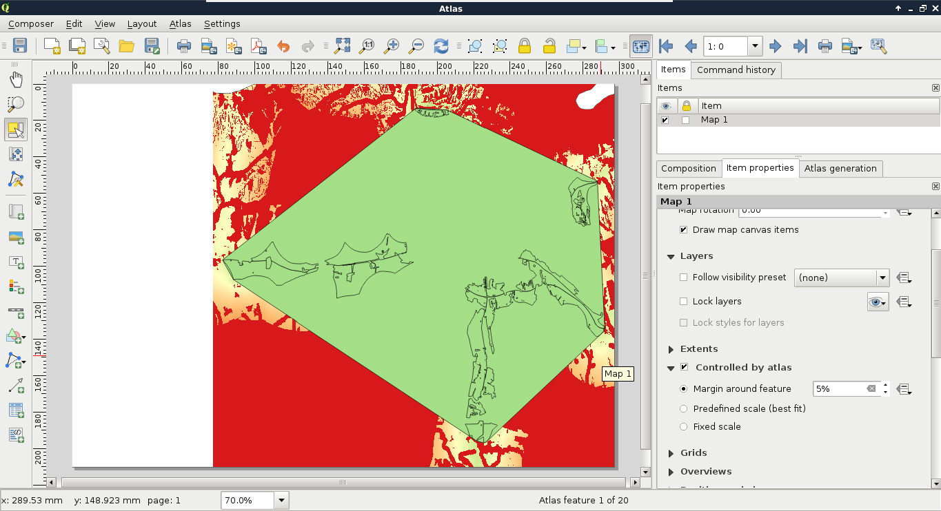
3. Select the map item, navigate to the Item properties tab, and check the Controlled by atlas box. This is an extension to the extent parameters, which automatically sets the data frame's extent to the extent of the current feature. Select the Margin around feature option.

4. Click on Preview Atlas on the main toolbar. You should be able to see the first page instantly, and navigate between the different pages with the blue arrows:

As the next step, we should style our layers in a way that they create an aesthetic composition in our atlas. For example, we should make the convex hull invisible, and remove the fills from the suitable sites:

1. Open the Properties | Style menu of the suitable sites layer, and select Rule-based styling.
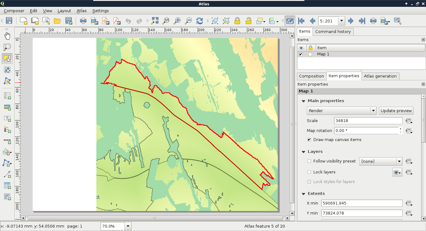
2. Modify the existing rule. Name it selected, and create an expression to show the current atlas feature if it is not the convex hull. Such an expression is "id" > 0 AND @atlas_featureid = $id, hence, the convex hull has an ID of 0. Style it with only an outline (Outline: Simple line), and apply a wide, colored line style.

3. Add a new rule. Name it not selected, and create an expression to show every feature besides the current atlas feature and the convex hull. The correct expression is "id" > 0 AND @atlas_featureid != $id. Style them with a narrow black outline.
4. The dominance of zero values in the suitability layer distorts the look of the map. Classify zeros as null values by opening Properties | Transparency, and defining 0 in the Additional no data value field:

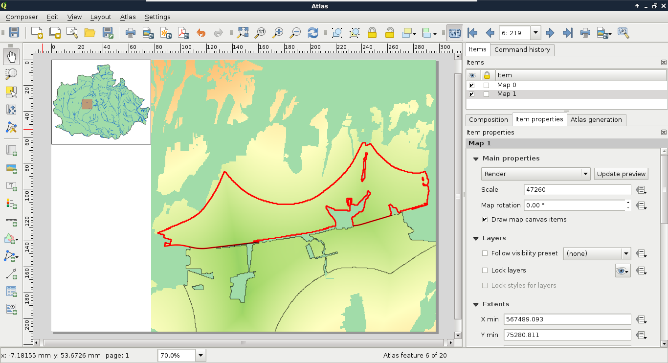
The second item we should add to our atlas is an overview map. This way, we can make sure we know where we are in the study area every time:

1. Add a new map frame with Add new map in one of the free corners of the canvas.
2. Style the layers in QGIS as you see fit. For the sake of simplicity, I added only the study area's polygon and the water layers.
3. After styling, go back to the composer, select the overview map, and check the Lock layers box.   
4. Position the map with Move item content in a way that the whole study area is in the frame. You can use the View extent in map canvas button as initial guidance.
5. In the Overviews section add a new item. Select the other map as Map frame.
6. Restore the initial layers in QGIS:

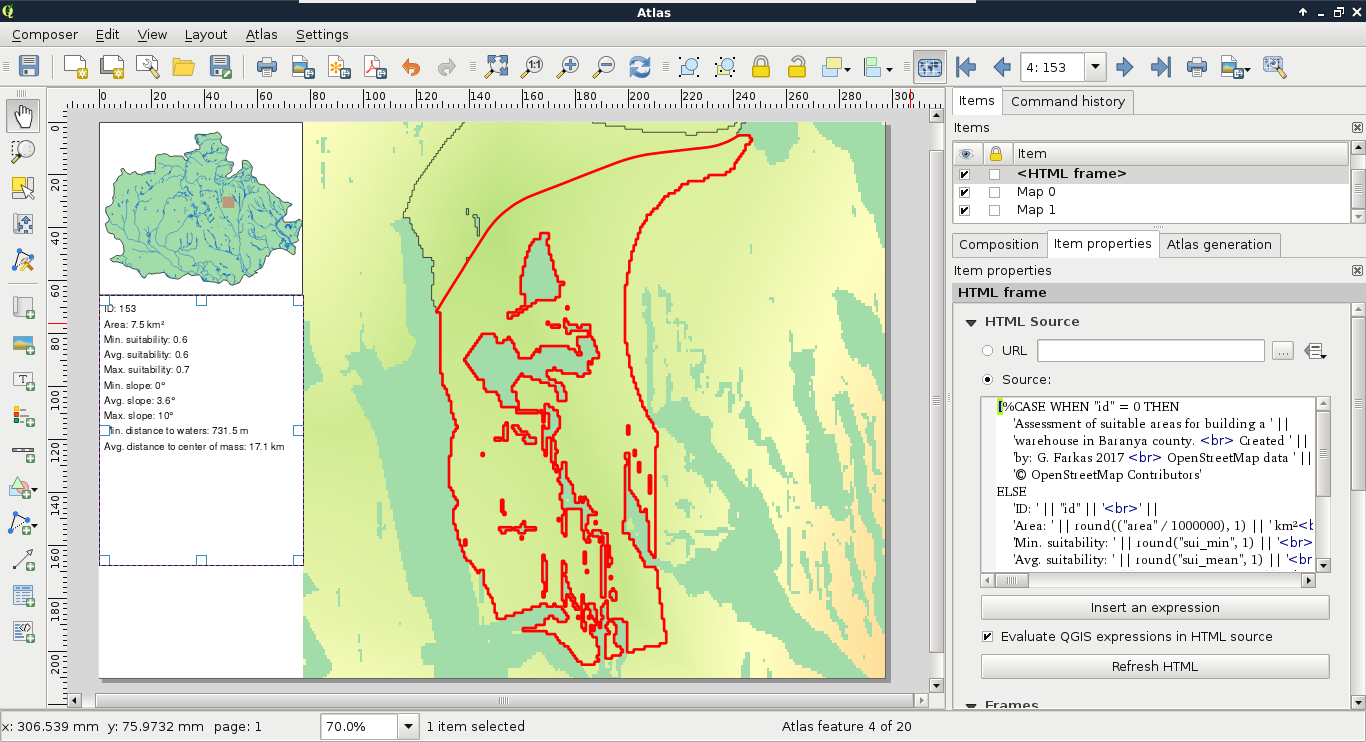
The next item we add is one of the most important parts of our atlas. It is the attributes of the atlas features. A simple way to achieve this would be to add an attribute table item with Add attribute table, although it cannot be customized enough to fit in our atlas. For these cases, QGIS's print composer offers a highly customizable item--the HTML frame. With that item, we can visualize any valid HTML document. Furthermore, we can use the expression builder to write expressions, which will be evaluated by QGIS and rendered in the HTML frame:

1. Add a new HTML frame with the Add HTML frame tool on the left toolbar.
2. In its Item properties dialog, select the Source radio button, and Evaluate QGIS expressions in HTML source box.

Now we just have to write our HTML containing the attributes of the features. A great thing in HTML is that plain text is a completely valid element. Therefore, we only need to know how to use one HTML element in order to fill our HTML frame, which is as follows:

• <br>: Inserts a line break in the HTML source.

The rest of the task is simple string concatenation (|| operator). We evaluate the attributes of the features (ID, area, and statistics), then concatenate them with the rest of the text and the <br> elements. Furthermore, as the HTML frame is an atlas-friendly item, the attributes of the current feature are automatically loaded, therefore, we can refer to the correct attribute with the name of the column. Finally, as the statistical indices are quite long, we should round them off with the round function. We can also divide the area by 1000000 to get the values in km²:

    [%'ID: ' || "id" || '<br>' ||
    'Area: ' || round(("area" / 1000000), 1) || ' km²<br>' ||
    'Min. suitability: ' || round("sui_min", 1) || '<br>' ||
    'Avg. suitability: ' || round("sui_mean", 1) || '<br>' ||
    'Max. suitability: ' || round("sui_max", 1) || '<br>' ||
    'Min. slope: ' || round("slp_min", 1) || '°<br>' ||
    'Avg. slope: ' || round("slp_mean", 1) || '°<br>' ||
    'Max. slope: ' || round("slp_max", 1) || '°<br>' ||
    'Min. distance to waters: ' || round("w_min", 1) || ' m<br>' ||
    'Avg. distance to center of mass:
     ' || round(("mc_mean" / 1000), 1) || ' km'%]

We should expand our expression a little bit. Although it shows the attributes of the atlas features nicely, we get a bunch of irrelevant numbers on the first page. Instead of visualizing them, we should print the title of the project, and the attributions on the first page. We can easily do this by extending our expression with the CASE conditional operator. We just have to specify the ID of the convex hull in the CASE clause, and put the attributes of the atlas features in the ELSE clause:

    [%CASE WHEN "id" = 0 THEN
     'Assessment of suitable areas for building a ' || 
     'warehouse in Baranya county. <br> Created ' || 
     'by: G. Farkas 2017 <br> OpenStreetMap data ' || 
     '© OpenStreetMap Contributors'
    ELSE
     'ID: ' || "id" || '<br>' ||
     'Area: ' || round(("area" / 1000000), 1) || ' km²<br>' ||
     'Min. suitability: ' || round("sui_min", 1) || '<br>' ||
     'Avg. suitability: ' || round("sui_mean", 1) || '<br>' ||
     'Max. suitability: ' || round("sui_max", 1) || '<br>' ||
     'Min. slope: ' || round("slp_min", 1) || '°<br>' ||
     'Avg. slope: ' || round("slp_mean", 1) || '°<br>' ||
     'Max. slope: ' || round("slp_max", 1) || '°<br>' ||
     'Min. distance to waters: ' || round("w_min", 1) || ' m<br>' ||
     'Avg. distance to center of mass: ' || round(("mc_mean" / 1000),
     1) || ' km'
    END%]

Now we can see our attributes when we focus on a feature, while the overview page shows only attribution:

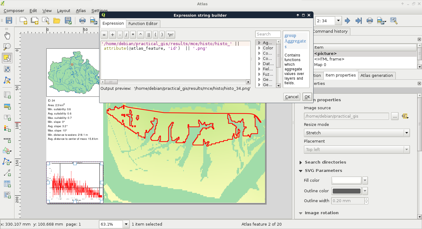
The final item we should add to our atlas is an image showing histograms. With data-defined override, we can get the correct histogram of every atlas feature if they are saved in the same folder, and contain the IDs of the features in their names:

1. Add a new image item with the Add image tool.
2. Choose the Data defined override button next to the Image source field, and select the Edit option.
3. Create an expression which returns the correct histogram file for every atlas feature. My expression is '/home/debian/practical_gis/results/mce/histo/histo_' || attribute(@atlas_feature, 'id') || '.png'. Note that the current atlas feature is not evaluated in a data-defined override (that is, we cannot access its attributes directly).

When we see our composition, we will be able to see some histograms, if we have them saved as images:

The only thing left to do is to export our atlas. By selecting the Export Atlas as Images button on the main toolbar, we can see that the atlas can be exported in image, SVG, and PDF formats. The most convenient way of exporting is to save the entire atlas in a single PDF, where every atlas page is rendered on a separate page:

1. Select the Atlas generation tab in the right panel.
2. Check the Single file export when possible box.
3. Save the atlas as a PDF with Export Atlas as Images | Export Atlas as PDF.