The easiest way to carry out a proximity analysis using rasters is GDAL's Proximity tool in QGIS. The tool requires a raster layer where features are described by cell values greater than zero. It takes the input raster, and creates the proximity grid--a raster with the same extent and resolution filled with distances from cells with values greater than zero. The behavior of the Proximity tool implies the following two things:

• We need to rasterize our input features
• We need to supply our rasterized features in a raster map covering our study area

As we've already found out, we can supply an existing raster layer to the Rasterize tool:

1. Select one of the factor inputs (like waterways, mean_coordinates, and so on).
2. Create a constant raster (a raster, where every cell has a same value) with the tool QGIS geolagorithms | Raster tools | Create constant raster layer. Supply the value of 0, and the constraints layer as a reference. Save it using the name of the selected factor.
3. Use the Rasterize tool with the selected factor's vector layer and the constant raster map created in the previous step.

4. Use the Raster | Analysis | Proximity tool to calculate the distances between zero and non-zero cells. The default distance units of GEO is sufficient, as it will assign values based on great-circle distances in meters. Save the result as a new file in a temporary folder.
5. Clip the result to the study area using Raster | Extraction | Clipper. Use the already extracted study area as a mask layer. Specify to cut the extent to the outline of the mask layer. Specify -1 as No data value, as 0 represents valuable information for the analysis.
6. Remove the temporary layer.
7. Repeat the steps with every input factor.

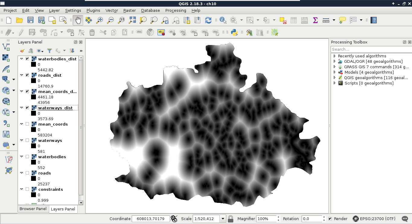
The distance matrices visualized in QGIS should have a peculiar texture slightly resembling a beehive:

Now that we have the distance matrices we will use for our factors, we can get rid of the intermediary data (that is, vectors and rasterized features). The next problem is that we have a single criterion in two different layers. We need distances from waters, although we have distances from rivers and lakes separately. As both of them form the same preference, and their units are the same (that is, they are on the same scale), we can use set operations to make a single map out of them. The two essential set operations for non-binary raster layers A and B using the same scale look like the following:

• Intersection (min(A, B)): The minimum of the two values define their intersection. For example, if we have a value of 10% for earthquake risk and a value of 30% for flood risk, the intersection, that is the risk of floods and earthquakes is 10% (not at the same time, though--that is an entirely different concept).
• Union (max(A, B)): The maximum of the two values define their union. If we have the same values as in the previous example, the risk of floods or earthquakes is 30%.

For creating the final water distance map, we need the intersection of the waterways and waterbodies layers. Unfortunately, we do not have minimum and maximum operators in QGIS's raster calculator. On the other hand, with a little logic, we can get the same result. All we have to do is composite two expressions in a way that they form an if-else clause:

    ("waterbodies_dist@1" <= "waterways_dist@1") * "waterbodies_dist@1"
     + ("waterbodies_dist@1" > "waterways_dist@1") * "waterways_dist@1"

This preceding expression can be read as follows:

• If cell values from waterbodies_dist are equal or smaller than cell values from weterways_dist, return one, otherwise return zero. Multiply that return value with the waterbodies_dist layer's cell value.
• If cell values from waterbodies_dist is larger than cell values from waterways_dist, return one, otherwise return zero. Multiply that return value with the waterways_dist layer's cell value.
• Add the two values together:

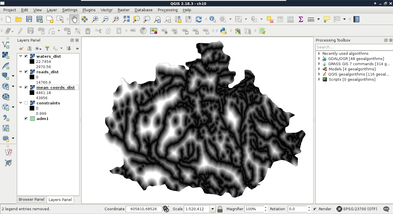
As we have the final distance layer for waters, the waterways and waterbodies layers are now obsolete, and we can safely remove them.