When it comes to web mapping and vector data, one of the most popular formats is GeoJSON. GeoJSON extends JSON, which is basically JavaScript's number one storage format. JSON is created to be concise while still able to represent almost every type in JavaScript. Therefore, we can save the states of web applications, for example, in order to resume them later. GeoJSON is also a concise format that can represent the basic geometry types and can be parsed by JavaScript easily. The only problem is that we have to load our GeoJSON files in our script. Although Leaflet knows how to handle GeoJSON objects, to load external content on the fly, we need to understand yet another concept--AJAX. On the other hand, there is a Leaflet plugin that can automatically load the content of a GeoJSON file with only URL. Let's create our third map using this plugin:
- Open QGIS and load the constrained houses layer. Export it with Save As. Choose the GeoJSON format and a CRS of WGS 84 (EPSG:4326). Name it houses.geojson and export it directly into the web server's root folder.
- Using Leaflet's plugin list, look for the Leaflet Ajax plugin. The link will lead to the GitHub page where the code is maintained. Click on the releases tab, which will navigate you to the release page of the plugin directly at https://github.com/calvinmetcalf/leaflet-ajax/releases.
- Download the latest release by clicking on the zip link under it. The archive comes with the source files and the debug version, which we do not need. Extract only the dist/leaflet.ajax.min.js file next to the Leaflet library.
- Edit the map.html file and include this new script in the <head> section after the Leaflet <script> element. As this is an extension, it needs Leaflet to be set up when it loads:
        <script src="leaflet/leaflet.ajax.min.js"
         type="text/javascript"></script>
- Create a new method for the third button in the maps object. The method should create a new map centered on the settlement we analyzed in Chapter 8, Spatial Analysis in QGIS:
        map = L.map('map', {
         center: [46.08, 18.24],
         zoom: 12
        });
- Add an OpenStreetMap base layer to the map, just like we did previously:
        L.tileLayer(
         'http://{s}.tile.openstreetmap.org/
         {z}/{x}/{y}.png').addTo(map);
- Add a new GeoJSON layer using AJAX with the L.geoJson.ajax function. It needs a relative path string as a parameter pointing to the GeoJSON file:
L.geoJson.ajax('houses.geojson').addTo(map);
If we click on the third button after refreshing the page, we can see our houses on the map:
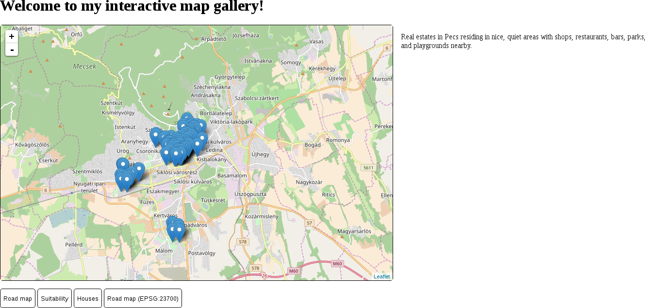
As we can see, Leaflet loads vector points as marker images by default. When we load some lines or polygons, it simply renders it as QGIS or GeoServer did. Let's load some polygons, but with WFS this time. Using WFS requests is another unsupported feature in Leaflet, which we can still use with another extension:
- Look for the plugin called Leaflet-WFST in the plugin list of Leaflet's page. The link will open the plugin's GitHub repository, where the plugin can be downloaded in the releases page. Download the latest release by clicking on the Source code (zip) button.
- Similarly to the previous plugin, we only need the minified version of the library and can discard the source files. Extract dist/Leaflet-WFST.min.js next to the Leaflet library in the web server's folder.
- Include this plugin in the map.html file's <head> section after Leaflet:
        <script src="leaflet/Leaflet-WFST.min.js"
         type="text/javascript"></script>
- In map.js, remove the tile layer containing our suitable areas from the suitability method of the maps object.
- Create a WFS layer instead. A simple WFS layer can be created with the L.wfs function. Unlike the previous functions, it only requires an object as a single parameter, and the object should contain the URL pointing at the OWS server with a url key. There are three more required parameters: typeNS with the queried workspace's name in GeoServer, typeName with the layer's name, and geometryField with the layer's geometry column. The default geometry column in GeoServer is the_geom:
        L.wfs({
         url: 'http://localhost:8080/geoserver/ows',
         typeNS: 'practical_gis',
         typeName: 'suitable',
         geometryField: 'the_geom'
        }).addTo(map);
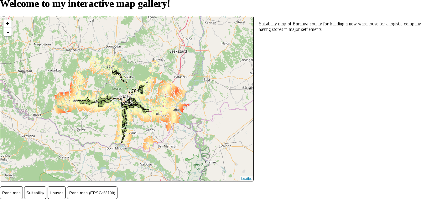
If we display our suitability map, we can see the OSM base layer and the suitability layer, but no polygons. What happened? You might have already opened the developer tools for potential error messages and seen a message similar to the following:
        XMLHttpRequest cannot load http://localhost:8080/geoserver/ows?.
         No 'Access-Control-Allow-Origin' header is present on the
         requested resource. Origin 'http://localhost' is therefore
         not allowed access.
We stumbled upon two very characteristic concepts of web development--same-origin policy and CORS (cross-origin resource sharing). The same-origin policy is a security measure that prevents browsers from mixing content from different servers. The path of the first document a web client loads determines the origin. From then on, the same-origin policy prevents the browser from loading anything that is not on exactly the same domain and exactly the same port. There are, of course, exceptions handled by CORS. These exceptions are typically scripts linked in <script> elements, stylesheets linked in <link> elements, images and other media, embedded content in <iframe> elements, and web fonts.
One of the things that the same-origin policy is always applied to is AJAX calls. WFS features, just like our GeoJSON file, are requested using AJAX, therefore the same-origin policy applies. The problem is that our GeoServer listens on and responds to port 8080, while our origin is at port 80. In the end, our web page cannot request resources other than images from GeoServer. The solution is simple; CORS can be enabled for any kind of resource on the server side using special headers in server responses. Enabling CORS in our GeoServer is slightly more complicated, though:
- Edit the webapps/geoserver/WEB-INF/web.xml file in GeoServer's folder.
- Look for the cross-origin, <filter>, and <filter-mapping> elements. There is a comment above them that states Uncomment following filter to enable CORS.
- Uncomment the elements by removing the <!-- and --> XML comment symbols around them.
- GeoServer's Jetty version does not have the required code to apply CORS headers on responses bundled by default. We have to download and install it manually. Get the Jetty version used by GeoServer by looking in the lib folder of GeoServer (not webapps/geoserver/WEB-INF/lib).
- The majority of the Java files starting with jetty contain Jetty's version number (for example, jetty-http-9.2.13.v20150730.jar).
- The Java file containing the required code for CORS headers is called jetty-servlets. Download the jar file with the appropriate version from http://central.maven.org/maven2/org/eclipse/jetty/jetty-servlets/. For example, for version 9.2.13.v20150730, you have to click on the corresponding version link and download the file named jetty-servlets-9.2.13.v20150730.jar by clicking on the file's link.
- Copy the downloaded file to webapps/geoserver/WEB-INF/lib in GeoServer's folder and restart GeoServer.
- After GeoServer runs, display the suitability map again to see our polygons: