Differences in x64 Architecture

The following are the most important differences between Windows 64-bit and 32-bit architecture:

All addresses and pointers are 64 bits.
All general-purpose registers—including RAX, RBX, RCX, and so on—have increased in size, although the 32-bit versions can still be accessed. For example, the RAX register is the 64-bit version of the EAX register.
Some of the general-purpose registers (RDI, RSI, RBP, and RSP) have been extended to support byte accesses, by adding an L suffix to the 16-bit version. For example, BP normally accesses the lower 16 bits of RBP; now, BPL accesses the lowest 8 bits of RBP.
The special-purpose registers are 64-bits and have been renamed. For example, RIP is the 64-bit instruction pointer.
There are twice as many general-purpose registers. The new registers are labeled R8 though R15. The DWORD (32-bit) versions of these registers can be accessed as R8D, R9D, and so on. WORD (16-bit) versions are accessed with a W suffix (R8W, R9W, and so on), and byte versions are accessed with an L suffix (R8L, R9L, and so on).

x64 also supports instruction pointer–relative data addressing. This is an important difference between x64 and x86 in relation to PIC and shellcode. Specifically, in x86 assembly, anytime you want to access data at a location that is not an offset from a register, the instruction must store the entire address. This is called absolute addressing. But in x64 assembly, you can access data at a location that is an offset from the current instruction pointer. The x64 literature refers to this as RIP-relative addressing. Example 21-1 shows a simple C program that accesses a memory address.

Example 21-1. A simple C program with a data access

int x;
void foo() {
      int y = x;
      ...
}

The x86 assembly code for Example 21-1 references global data (the variable x). In order to access this data, the instruction encodes the 4 bytes representing the data’s address. This instruction is not position independent, because it will always access address 0x00403374, but if this file were to be loaded at a different location, the instruction would need to be modified so that the mov instruction accessed the correct address, as shown in Example 21-2.

Example 21-2. x86 assembly for the C program in Example 21-1

00401004 A1 ❶74 ❷33 ❸40 ❹00 mov     eax, dword_403374

You’ll notice that the bytes of the address are stored with the instruction at ❶, ❷, ❸, and ❹. Remember that the bytes are stored with the least significant byte first. The bytes 74, 33, 40, and 00 correspond to the address 0x00403374.

After recompiling for x64, Example 21-3 shows the same mov instruction that appears in Example 21-2.

Example 21-3. x64 assembly for Example 21-1

0000000140001058 8B 05 ❶A2 ❷D3 ❸00 ❹00 mov     eax, dword_14000E400

At the assembly level, there doesn’t appear to be any change. The instruction is still mov eax, dword_address, and IDA Pro automatically calculates the instruction’s address. However, the differences at the opcode level allow this code to be position-independent on x64, but not x86.

In the 64-bit version of the code, the instruction bytes do not contain the fixed address of the data. The address of the data is 14000E400, but the instruction bytes are A2 ❶, D3 ❷, 00 ❸, and 00 ❹, which correspond to the value 0x0000D3A2.

The 64-bit instruction stores the address of the data as an offset from the current instruction pointer, rather than as an absolute address, as stored in the 32-bit version. If this file were loaded at a different location, the instruction would still point to the correct address, unlike in the 32-bit version. In that case, if the file is loaded at a different address, the reference must be changed.

Instruction pointer–relative addressing is a powerful addition to the x64 instruction set that significantly decreases the number of addresses that must be relocated when a DLL is loaded. Instruction pointer–relative addressing also makes it much easier to write shellcode because it eliminates the need to obtain a pointer to EIP in order to access data. Unfortunately, this addition also makes it more difficult to detect shellcode, because it eliminates the need for a call/pop as discussed in Position-Independent Code. Many of those common shellcode techniques are unnecessary or irrelevant when working with malware written to run on the x64 architecture.

Differences in the x64 Calling Convention and Stack Usage

The calling convention used by 64-bit Windows is closest to the 32-bit fastcall calling convention discussed in Chapter 6. The first four parameters of the call are passed in the RCX, RDX, R8, and R9 registers; additional ones are stored on the stack.

Note

Most of the conventions and hints described in this section apply to compiler-generated code that runs on the Windows OS. There is no processor-enforced requirement to follow these conventions, but Microsoft’s guidelines for compilers specify certain rules in order to ensure consistency and stability. Beware, because hand-coded assembly and malicious code may disregard these rules and do the unexpected. As usual, investigate any code that doesn’t follow the rules.

In the case of 32-bit code, stack space can be allocated and unallocated in the middle of the function using push and pop instructions. However, in 64-bit code, functions cannot allocate any space in the middle of the function, regardless of whether they’re push or other stack-manipulation instructions.

Figure 21-1 compares the stack management of 32-bit and 64-bit code. Notice in the graph for a 32-bit function that the stack size grows as arguments are pushed on the stack, and then falls when the stack is cleaned up. Stack space is allocated at the beginning of the function, and moves up and down during the function call. When calling a function, the stack size grows; when the function returns, the stack size returns to normal. In contrast, the graph for a 64-bit function shows that the stack grows at the start of the function and remains at that level until the end of the function.

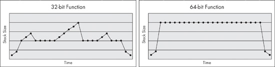
Figure 21-1. Stack size in the same function compiled for 32-bit and 64-bit architectures

The 32-bit compiler will sometimes generate code that doesn’t change the stack size in the middle of the function, but 64-bit code never changes the stack size in the middle of the function. Although this stack restriction is not enforced by the processor, the Microsoft 64-bit exception-handling model depends on it in order to function properly. Functions that do not follow this convention may crash or cause other problems if an exception occurs.

The lack of push and pop instructions in the middle of a function can make it more difficult for an analyst to determine how many parameters a function has, because there is no easy way to tell whether a memory address is being used as a stack variable or as a parameter to a function. There’s also no way to tell whether a register is being used as a parameter. For example, if ECX is loaded with a value immediately before a function call, you can’t tell if the register is loaded as a parameter or for some other reason.

Example 21-4 shows an example of the disassembly for a function call compiled for a 32-bit processor.

Example 21-4. Call to printf compiled for a 32-bit processor

004113C0  mov     eax, [ebp+arg_0]
004113C3  push    eax
004113C4  mov     ecx, [ebp+arg_C]
004113C7  push    ecx
004113C8  mov     edx, [ebp+arg_8]
004113CB  push    edx
004113CC  mov     eax, [ebp+arg_4]
004113CF  push    eax
004113D0  push    offset aDDDD_
004113D5  call    printf
004113DB  add     esp, 14h

The 32-bit assembly has five push instructions before the call to printf, and immediately after the call to printf, 0x14 is added to the stack to clean it up. This clearly indicates that there are five parameters being passed to the printf function.

Example 21-5 shows the disassembly for the same function call compiled for a 64-bit processor:

Example 21-5. Call to printf compiled for a 64-bit processor

0000000140002C96  mov     ecx, [rsp+38h+arg_0]
0000000140002C9A  mov     eax, [rsp+38h+arg_0]
0000000140002C9E ❶mov     [rsp+38h+var_18], eax
0000000140002CA2  mov     r9d, [rsp+38h+arg_18]
0000000140002CA7  mov     r8d, [rsp+38h+arg_10]
0000000140002CAC  mov     edx, [rsp+38h+arg_8]
0000000140002CB0  lea     rcx, aDDDD_
0000000140002CB7  call    cs:printf

In 64-bit disassembly, the number of parameters passed to printf is less evident. The pattern of load instructions in RCX, RDX, R8, and R9 appears to show parameters being moved into the registers for the printf function call, but the mov instruction at ❶ is not as clear. IDA Pro labels this as a move into a local variable, but there is no clear way to distinguish between a move into a local variable and a parameter for the function being called. In this case, we can just check the format string to see how many parameters are being passed, but in other cases, it will not be so easy.

Leaf and Nonleaf Functions

The 64-bit stack usage convention breaks functions into two categories: leaf and nonleaf functions. Any function that calls another function is called a nonleaf function, and all other functions are leaf functions.

Nonleaf functions are sometimes called frame functions because they require a stack frame. All nonleaf functions are required to allocate 0x20 bytes of stack space when they call a function. This allows the function being called to save the register parameters (RCX, RDX, R8, and R9) in that space, if necessary.

In both leaf and nonleaf functions, the stack will be modified only at the beginning or end of the function. These portions that can modify the stack frame are discussed next.

Prologue and Epilogue 64-Bit Code

Windows 64-bit assembly code has well-formed sections at the beginning and end of functions called the prologue and epilogue, which can provide useful information. Any mov instructions at the beginning of a prologue are always used to store the parameters that were passed into the function. (The compiler cannot insert mov instructions that do anything else within the prologue.) Example 21-6 shows an example of a prologue for a small function.

Example 21-6. Prologue code for a small function

00000001400010A0  mov     [rsp+arg_8], rdx
00000001400010A5  mov     [rsp+arg_0], ecx
00000001400010A9  push    rdi
00000001400010AA  sub     rsp, 20h

Here, we see that this function has two parameters: one 32-bit and one 64-bit. This function allocates 0x20 bytes from the stack, as required by all nonleaf functions as a place to provide storage for parameters. If a function has any local stack variables, it will allocate space for them in addition to the 0x20 bytes. In this case, we can tell that there are no local stack variables because only 0x20 bytes are allocated.

64-Bit Exception Handling

Unlike exception handling in 32-bit systems, structured exception handling in x64 does not use the stack. In 32-bit code, the fs:[0] is used as a pointer to the current exception handler frame, which is stored on the stack so that each function can define its own exception handler. As a result, you will often find instructions modifying fs:[0] at the beginning of a function. You will also find exploit code that overwrites the exception information on the stack in order to get control of the code executed during an exception.

Structured exception handling in x64 uses a static exception information table stored in the PE file and does not store any data on the stack. Also, there is an _IMAGE_RUNTIME_FUNCTION_ENTRY structure in the .pdata section for every function in the executable that stores the beginning and ending address of the function, as well as a pointer to exception-handling information for that function.

Previous Chapter

Why 64-Bit Malware?

Next Chapter

Windows 32-Bit on Windows 64-Bit