The most common anti-disassembly technique seen in the wild is two back-to-back conditional jump instructions that both point to the same target. For example, if a jz loc_512 is followed by jnz loc_512, the location loc_512 will always be jumped to. The combination of jz with jnz is, in effect, an unconditional jmp, but the disassembler doesn’t recognize it as such because it only disassembles one instruction at a time. When the disassembler encounters the jnz, it continues disassembling the false branch of this instruction, despite the fact that it will never be executed in practice.

The following code shows IDA Pro’s first interpretation of a piece of code protected with this technique:

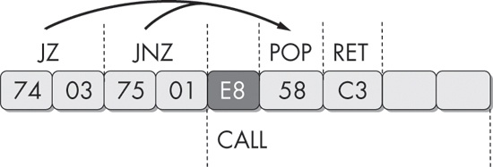
74 03                  jz      short near ptr loc_4011C4+1
75 01                  jnz     short near ptr loc_4011C4+1
                       loc_4011C4:                     ; CODE XREF: sub_4011C0
                                                       ; ❷sub_4011C0+2j
E8 58 C3 90 90        ❶call    near ptr 90D0D521h

In this example, the instruction immediately following the two conditional jump instructions appears to be a call instruction at ❶, beginning with the byte 0xE8. This is not the case, however, as both conditional jump instructions actually point 1 byte beyond the 0xE8 byte. When this fragment is viewed with IDA Pro, the code cross-references shown at ❷ loc_4011C4 will appear in red, rather than the standard blue, because the actual references point inside the instruction at this location, instead of the beginning of the instruction. As a malware analyst, this is your first indication that anti-disassembly may be employed in the sample you are analyzing.

The following is disassembly of the same code, but this time fixed with the D key, to turn the byte immediately following the jnz instruction into data, and the C key to turn the bytes at loc_4011C5 into instructions.

74 03                  jz      short near ptr loc_4011C5
75 01                  jnz     short near ptr loc_4011C5
         ; -------------------------------------------------------------------
E8                     db 0E8h
         ; -------------------------------------------------------------------
                       loc_4011C5:                     ; CODE XREF: sub_4011C0
                                                       ; sub_4011C0+2j
58                     pop     eax
C3                     retn

The column on the left in these examples shows the bytes that constitute the instruction. Display of this field is optional, but it’s important when learning anti-disassembly. To display these bytes (or turn them off), select Options ▶ General. The Number of Opcode Bytes option allows you to enter a number for how many bytes you would like to be displayed.

Figure 15-2 shows the sequence of bytes in this example graphically.

Figure 15-2. A jz instruction followed by a jnz instruction

Another anti-disassembly technique commonly found in the wild is composed of a single conditional jump instruction placed where the condition will always be the same. The following code uses this technique:

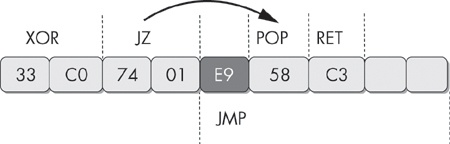
33 C0                  xor     eax, eax
74 01                  jz      short near ptr loc_4011C4+1
        loc_4011C4:                             ; CODE XREF: 004011C2j
                                                ; DATA XREF: .rdata:004020ACo
E9 58 C3 68 94         jmp     near ptr 94A8D521h

Notice that this code begins with the instruction xor eax, eax. This instruction will set the EAX register to zero and, as a byproduct, set the zero flag. The next instruction is a conditional jump that will jump if the zero flag is set. In reality, this is not conditional at all, since we can guarantee that the zero flag will always be set at this point in the program.

As discussed previously, the disassembler will process the false branch first, which will produce conflicting code with the true branch, and since it processed the false branch first, it trusts that branch more. As you’ve learned, you can use the D key on the keyboard while your cursor is on a line of code to turn the code into data, and pressing the C key will turn the data into code. Using these two keyboard shortcuts, a malware analyst could fix this fragment and have it show the real path of execution, as follows:

33 C0                  xor     eax, eax
74 01                  jz      short near ptr loc_4011C5
        ; --------------------------------------------------------------------
E9                     db 0E9h
        ; --------------------------------------------------------------------
        loc_4011C5:                             ; CODE XREF: 004011C2j
                                                ; DATA XREF: .rdata:004020ACo
58                     pop     eax
C3                     retn

In this example, the 0xE9 byte is used exactly as the 0xE8 byte in the previous example. E9 is the opcode for a 5-byte jmp instruction, and E8 is the opcode for a 5-byte call instruction. In each case, by tricking the disassembler into disassembling this location, the 4 bytes following this opcode are effectively hidden from view. Figure 15-3 shows this example graphically.

Figure 15-3. False conditional of xor followed by a jz instruction

In the previous sections, we examined code that was improperly disassembled by the first attempt made by the disassembler, but with an interactive disassembler like IDA Pro, we were able to work with the disassembly and have it produce accurate results. However, under some conditions, no traditional assembly listing will accurately represent the instructions that are executed. We use the term impossible disassembly for such conditions, but the term isn’t strictly accurate. You could disassemble these techniques, but you would need a vastly different representation of code than what is currently provided by disassemblers.

The simple anti-disassembly techniques we have discussed use a data byte placed strategically after a conditional jump instruction, with the idea that disassembly starting at this byte will prevent the real instruction that follows from being disassembled because the byte that is inserted is the opcode for a multibyte instruction. We’ll call this a rogue byte because it is not part of the program and is only in the code to throw off the disassembler. In all of these examples, the rogue byte can be ignored.

But what if the rogue byte can’t be ignored? What if it is part of a legitimate instruction that is actually executed at runtime? Here, we encounter a tricky scenario where any given byte may be a part of multiple instructions that are executed. No disassembler currently on the market will represent a single byte as being part of two instructions, yet the processor has no such limitation.

Figure 15-4 shows an example. The first instruction in this 4-byte sequence is a 2-byte jmp instruction. The target of the jump is the second byte of itself. This doesn’t cause an error, because the byte FF is the first byte of the next 2-byte instruction, inc eax.

Figure 15-4. Inward-pointing jmp instruction

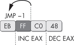
The predicament when trying to represent this sequence in disassembly is that if we choose to represent the FF byte as part of the jmp instruction, then it won’t be available to be shown as the beginning of the inc eax instruction. The FF byte is a part of both instructions that actually execute, and our modern disassemblers have no way of representing this. This 4-byte sequence increments EAX, and then decrements it, which is effectively a complicated NOP sequence. It could be inserted at almost any location within a program to break the chain of valid disassembly. To solve this problem, a malware analyst could choose to replace this entire sequence with NOP instructions using an IDC or IDAPython script that calls the PatchByte function. Another alternative is to simply turn it all into data with the D key, so that disassembly will resume as expected at the end of the 4 bytes.

For a glimpse of the complexity that can be achieved with these sorts of instruction sequences, let’s examine a more advanced specimen. Figure 15-5 shows an example that operates on the same principle as the prior one, where some bytes are part of multiple instructions.

Figure 15-5. Multilevel inward-jumping sequence

The first instruction in this sequence is a 4-byte mov instruction. The last 2 bytes have been highlighted because they are both part of this instruction and are also their own instruction to be executed later. The first instruction populates the AX register with data. The second instruction, an xor, will zero out this register and set the zero flag. The third instruction is a conditional jump that will jump if the zero flag is set, but it is actually unconditional, since the previous instruction will always set the zero flag. The disassembler will decide to disassemble the instruction immediately following the jz instruction, which will begin with the byte 0xE8, the opcode for a 5-byte call instruction. The instruction beginning with the byte E8 will never execute in reality.

The disassembler in this scenario can’t disassemble the target of the jz instruction because these bytes are already being accurately represented as part of the mov instruction. The code that the jz points to will always be executed, since the zero flag will always be set at this point. The jz instruction points to the middle of the first 4-byte mov instruction. The last 2 bytes of this instruction are the operand that will be moved into the register. When disassembled or executed on their own, they form a jmp instruction that will jump forward 5 bytes from the end of the instruction.

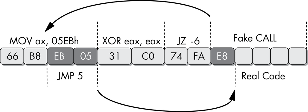
When first viewed in IDA Pro, this sequence will look like the following:

66 B8 EB 05            mov     ax, 5EBh
31 C0                  xor     eax, eax
74 FA                  jz      short near ptr sub_4011C0+2
                loc_4011C8:
E8 58 C3 90 90         call    near ptr 98A8D525h

Since there is no way to clean up the code so that all executing instructions are represented, we must choose the instructions to leave in. The net side effect of this anti-disassembly sequence is that the EAX register is set to zero. If you manipulate the code with the D and C keys in IDA Pro so that the only instructions visible are the xor instruction and the hidden instructions, your result should look like the following.

66                   byte_4011C0     db 66h
B8                                   db 0B8h
EB                                   db 0EBh
05                                   db    5
                ; ------------------------------------------------------------
31 C0                                xor     eax, eax
                ; ------------------------------------------------------------
74                                   db 74h
FA                                   db 0FAh
E8                                   db 0E8h
                ; ------------------------------------------------------------
58                                   pop     eax
C3                                   retn

This is a somewhat acceptable solution because it shows only the instructions that are relevant to understanding the program. However, this solution may interfere with analysis processes such as graphing, since it’s difficult to tell exactly how the xor instruction or the pop and retn sequences are executed. A more complete solution would be to use the PatchByte function from the IDC scripting language to modify remaining bytes so that they appear as NOP instructions.

This example has two areas of undisassembled bytes that we need to convert into NOP instructions: 4 bytes starting at memory address 0x004011C0 and 3 bytes starting at memory address 0x004011C6. The following IDAPython script will convert these bytes into NOP bytes (0x90):

def NopBytes(start, length):
   for i in range(0, length):
     PatchByte(start + i, 0x90)
   MakeCode(start)

NopBytes(0x004011C0, 4)
NopBytes(0x004011C6, 3)

This code takes the long approach by making a utility function called NopBytes to NOP-out a range of bytes. It then uses that utility function against the two ranges that we need to fix. When this script is executed, the resulting disassembly is clean, legible, and logically equivalent to the original:

90                       nop
90                       nop
90                       nop
90                       nop
31 C0                    xor     eax, eax
90                       nop
90                       nop
90                       nop
58                       pop     eax
C3                       retn

The IDAPython script we just crafted worked beautifully for this scenario, but it is limited in its usefulness when applied to new challenges. To reuse the previous script, the malware analyst must decide which offsets and which length of bytes to change to NOP instructions, and manually edit the script with the new values.

With a little IDA Python knowledge, we can develop a script that allows malware analysts to easily NOP-out instructions as they see fit. The following script establishes the hotkey ALT-N. Once this script is executed, whenever the user presses ALT-N, IDA Pro will NOP-out the instruction that is currently at the cursor location. It will also conveniently advance the cursor to the next instruction to facilitate easy NOP-outs of large blocks of code.

import idaapi

idaapi.CompileLine('static n_key() { RunPythonStatement("nopIt()"); }')

AddHotkey("Alt-N", "n_key")

def nopIt():

      start = ScreenEA()
      end = NextHead(start)
      for ea in range(start, end):
            PatchByte(ea, 0x90)
      Jump(end)
      Refresh()