The linear-disassembly strategy iterates over a block of code, disassembling one instruction at a time linearly, without deviating. This basic strategy is employed by disassembler writing tutorials and is widely used by debuggers. Linear disassembly uses the size of the disassembled instruction to determine which byte to disassemble next, without regard for flow-control instructions.

The following code fragment shows the use of the disassembly library libdisasm (http://sf.net/projects/bastard/files/libdisasm/) to implement a crude disassembler in a handful of lines of C using linear disassembly:

char buffer[BUF_SIZE];
int position = 0;

while (position < BUF_SIZE) {
   x86_insn_t insn;
   int size = x86_disasm(buf, BUF_SIZE, 0, position, &insn);

   if (size != 0) {
      char disassembly_line[1024];
        x86_format_insn(&insn, disassembly_line, 1024, intel_syntax);
        printf("%s\n", disassembly_line);
      ❶position += size;
   } else {
        /* invalid/unrecognized instruction */
      ❷position++;
      }
}
x86_cleanup();

In this example, a buffer of data named buffer contains instructions to be disassembled. The function x86_disasm will populate a data structure with the specifics of the instruction it just disassembled and return the size of the instruction. The loop increments the position variable by the size value ❶ if a valid instruction was disassembled; otherwise, it increments by one ❷.

This algorithm will disassemble most code without a problem, but it will introduce occasional errors even in nonmalicious binaries. The main drawback to this method is that it will disassemble too much code. The algorithm will keep blindly disassembling until the end of the buffer, even if flow-control instructions will cause only a small portion of the buffer to execute.

In a PE-formatted executable file, the executable code is typically contained in a single section. It is reasonable to assume that you could get away with just applying this linear-disassembly algorithm to the .text section containing the code, but the problem is that the code section of nearly all binaries will also contain data that isn’t instructions.

One of the most common types of data items found in a code section is a pointer value, which is used in a table-driven switch idiom. The following disassembly fragment (from a nonlinear disassembler) shows a function that contains switch pointers immediately following the function code.

          jmp     ds:off_401050[eax*4] ; switch jump

          ; switch cases omitted ...

          xor     eax, eax
          pop     esi
          retn
; ---------------------------------------------------------------------------
off_401050  ❶dd offset loc_401020    ; DATA XREF: _main+19r
             dd offset loc_401027    ; jump table for switch statement
             dd offset loc_40102E
             dd offset loc_401035

The last instruction in this function is retn. In memory, the bytes immediately following the retn instruction are the pointer values beginning with 401020 at ❶, which in memory will appear as the byte sequence 20 10 40 00 in hex. These four pointer values shown in the code fragment make up 16 bytes of data inside the .text section of this binary. They also happen to disassemble to valid instructions. The following disassembly fragment would be produced by a linear-disassembly algorithm when it continues disassembling instructions beyond the end of the function:

and [eax],dl
inc eax
add [edi],ah
adc [eax+0x0],al
adc cs:[eax+0x0],al
xor eax,0x4010

Many of instructions in this fragment consist of multiple bytes. The key way that malware authors exploit linear-disassembly algorithms lies in planting data bytes that form the opcodes of multibyte instructions. For example, the standard local call instruction is 5 bytes, beginning with the opcode 0xE8. If the 16 bytes of data that compose the switch table end with the value 0xE8, the disassembler would encounter the call instruction opcode and treat the next 4 bytes as an operand to that instruction, instead of the beginning of the next function.

Linear-disassembly algorithms are the easiest to defeat because they are unable to distinguish between code and data.

A more advanced category of disassembly algorithms is the flow-oriented disassembler. This is the method used by most commercial disassemblers such as IDA Pro.

The key difference between flow-oriented and linear disassembly is that the disassembler doesn’t blindly iterate over a buffer, assuming the data is nothing but instructions packed neatly together. Instead, it examines each instruction and builds a list of locations to disassemble.

The following fragment shows code that can be disassembled correctly only with a flow-oriented disassembler.

                test    eax, eax
               ❶jz      short loc_1A
               ❷push    Failed_string
               ❸call    printf
               ❹jmp     short loc_1D
; ---------------------------------------------------------------------------
Failed_string:  db 'Failed',0
; ---------------------------------------------------------------------------
loc_1A: ❺
                xor     eax, eax
loc_1D:
                retn

This example begins with a test and a conditional jump. When the flow-oriented disassembler reaches the conditional branch instruction jz at ❶, it notes that at some point in the future it needs to disassemble the location loc_1A at ❺. Because this is only a conditional branch, the instruction at ❷ is also a possibility in execution, so the disassembler will disassemble this as well.

The lines at ❷ and ❸ are responsible for printing the string Failed to the screen. Following this is a jmp instruction at ❹. The flow-oriented disassembler will add the target of this, loc_1D, to the list of places to disassemble in the future. Since jmp is unconditional, the disassembler will not automatically disassemble the instruction immediately following in memory. Instead, it will step back and check the list of places it noted previously, such as loc_1A, and disassemble starting from that point.

In contrast, when a linear disassembler encounters the jmp instruction, it will continue blindly disassembling instructions sequentially in memory, regardless of the logical flow of the code. In this case, the Failed string would be disassembled as code, inadvertently hiding the ASCII string and the last two instructions in the example fragment. For example, the following fragment shows the same code disassembled with a linear-disassembly algorithm.

                test    eax, eax
                jz      short near ptr loc_15+5
                push    Failed_string
                call    printf
                jmp     short loc_15+9
Failed_string:
                inc     esi
                popa
loc_15:
                imul    ebp, [ebp+64h], 0C3C03100h

In linear disassembly, the disassembler has no choice to make about which instructions to disassemble at a given time. Flow-oriented disassemblers make choices and assumptions. Though assumptions and choices might seem unnecessary, simple machine code instructions are complicated by the addition of problematic code aspects such as pointers, exceptions, and conditional branching.

Conditional branches give the flow-oriented disassembler a choice of two places to disassemble: the true or the false branch. In typical compiler-generated code, there would be no difference in output if the disassembler processes the true or false branch first. In handwritten assembly code and anti-disassembly code, however, the two branches can often produce different disassembly for the same block of code. When there is a conflict, most disassemblers trust their initial interpretation of a given location first. Most flow-oriented disassemblers will process (and thus trust) the false branch of any conditional jump first.

Figure 15-1 shows a sequence of bytes and their corresponding machine instructions. Notice the string hello in the middle of the instructions. When the program executes, this string is skipped by the call instruction, and its 6 bytes and NULL terminator are never executed as instructions.

Figure 15-1. call instruction followed by a string

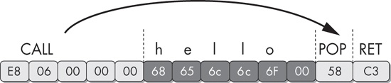
The call instruction is another place where the disassembler must make a decision. The location being called is added to the future disassembly list, along with the location immediately after the call. Just as with the conditional jump instructions, most disassemblers will disassemble the bytes after the call instruction first and the called location later. In handwritten assembly, programmers will often use the call instruction to get a pointer to a fixed piece of data instead of actually calling a subroutine. In this example, the call instruction is used to create a pointer for the string hello on the stack. The pop instruction following the call then takes this value off the top of the stack and puts it into a register (EAX in this case).

When we disassemble this binary with IDA Pro, we see that it has produced disassembly that is not what we expected:

E8 06 00 00 00       call    near ptr loc_4011CA+1
68 65 6C 6C 6F      ❶push    6F6C6C65h

                     loc_4011CA:
00 58 C3             add     [eax-3Dh], bl

As it turns out, the first letter of the string hello is the letter h, which is 0x68 in hexadecimal. This is also the opcode of the 5-byte instruction ❶ push DWORD. The null terminator for the hello string turned out to also be the first byte of another legitimate instruction. The flow-oriented disassembler in IDA Pro decided to process the thread of disassembly at ❶ (immediately following the call instruction) before processing the target of the call instruction, and thus produced these two erroneous instructions. Had it processed the target first, it still would have produced the first push instruction, but the instruction following the push would have conflicted with the real instructions it disassembled as a result of the call target.

If IDA Pro produces inaccurate results, you can manually switch bytes from data to instructions or instructions to data by using the C or D keys on the keyboard, as follows:

Here is the same function after manual cleanup:

E8 06 00 00 00                       call    loc_4011CB
68 65 6C 6C 6F 00    aHello          db 'hello',0
                                     loc_4011CB:
58                                   pop     eax
C3                                   retn