Virtual vs. Nonvirtual Functions

A virtual function is one that can be overridden by a subclass and whose execution is determined at runtime. If a function is defined within a parent class and a function with the same name is defined in a child class, the child class’s function overrides the parent’s function.

Several popular programming models use this functionality in order to greatly simplify complex programming tasks. To illustrate why this is useful, return to the socket example in Example 20-5. There, we have code that is going to sendData over the network, and we want it to be able to send data via TCP and UDP. One easy way to accomplish this is to create a parent class called Socket with a virtual function called sendData. Then we have two children classes called UDPSocket and TCPSocket, which override the sendData function to send the data over the appropriate protocol.

In the code that uses the socket, we create an object of type Socket, and create whichever socket we are using in this instance. Each time we call the sendData function, the sendData function will be called from the proper subclass of Socket, whether UDPSocket or TCPSocket, based on which type of Socket object was originally created.

The biggest advantage here is that if a new protocol—QDP, for example—is invented, you simply create a new QDPSocket class, and then change the line of code where the object is created. Then all calls to sendData will call the new QDPSocket version of sendData without the need to change all the calls individually.

In the case of nonvirtual functions, the function to be executed is determined at compile time. If the object is an instance of the parent class, the parent class’s function will be called, even if the object at runtime belongs to the child class. When a virtual function is called on an object of the child class, the child class’s version of the function may be called, if the object is typed as an instance of the parent class.

Table 20-1 shows a code snippet that will execute differently if the function is virtual or nonvirtual.

Table 20-1. Source Code Example for Virtual Functions

Non-virtual function	Virtual function
class A { public: void foo() { printf("Class A\n"); } }; class B : public A { public: void foo() { printf("Class B\n"); } }; void g(A& arg) { arg.foo(); } int _tmain(int argc, _TCHAR* argv[]) { B b; A a; g(b); return 0; }	class A { public: ❷virtual void foo() { printf("Class A\n"); } }; class B : public A { public: ❶virtual void foo() { printf("Class B\n"); } }; void g(A& arg) { ❸arg.foo(); } int _tmain(int argc, _TCHAR* argv[]) { B b; A a; g(b); return 0; }

Non-virtual function

Virtual function

class A {
public:
      void foo() {
            printf("Class A\n");
      }
};

class B : public A {
public:
      void foo() {
            printf("Class B\n");
      }
};

void g(A& arg) {
      arg.foo();
}

int _tmain(int argc, _TCHAR* argv[])
{
      B b;
      A a;
      g(b);
      return 0;
}

class A {
public:
     ❷virtual void foo() {
            printf("Class A\n");
      }
};

class B : public A {
public:
     ❶virtual void foo() {
            printf("Class B\n");
      }
};

void g(A& arg) {
     ❸arg.foo();
}

int _tmain(int argc, _TCHAR* argv[])
{
      B b;
      A a;
      g(b);
      return 0;
}

The code contains two classes: class A and class B. The class B class overrides the foo method from class A. The code also contains a function to call the foo method from outside either class. If the function is not declared as virtual, it will print “Class A.” If it is declared as virtual, it will print “Class B.” The code on either side is identical except for the virtual keywords at ❶ and ❷.

In the case of nonvirtual functions, the determination of which function to call is made at compile time. In the two code samples in Example 20-6, when this code is compiled, the object at ❸ is of class A. While the object at ❸ could be a subclass of class A, at compile time, we know that it is an object of class A, and the foo function for class A is called. This is why the code on the left will print “Class A.”

In the case of virtual functions, the determination of which function to call is made at runtime. If a class A object is called at runtime, then the class A version of the function is called. If the object is of class B, then the class B function is called. This is why the code on the right will print “Class B.”

This functionality is often referred to as polymorphism. The biggest advantage to polymorphism is that it allows objects that perform different functionality to share a common interface.

Use of Vtables

The C++ compiler will add special data structures when it compiles code to support virtual functions. These data structures are called virtual function tables, or vtables. These tables are simply arrays of function pointers. Each class using virtual functions has its own vtable, and each virtual function in a class has an entry in the vtable.

Table 20-2 shows a disassembly of g function from the two code snippets in Table 20-1. On the left is the nonvirtual function call to foo, and on the right is the virtual call.

Table 20-2. Assembly Code of the Example from Table 20-1

Non-virtual function call	Virtual function call
00401000 push ebp 00401001 mov ebp, esp 00401003 mov ecx, [ebp+arg_0] 00401006 call sub_401030 0040100B pop ebp 0040100C retn	00401000 push ebp 00401001 mov ebp, esp 00401003 mov ❶eax, [ebp+arg_0] 00401006 mov ❷edx, [eax] 00401008 mov ecx, [ebp+arg_0] 0040100B mov eax, [edx] 0040100D call eax 0040100F pop ebp 00401010 retn

Non-virtual function call

Virtual function call

00401000   push    ebp
00401001   mov     ebp, esp
00401003   mov     ecx, [ebp+arg_0]
00401006   call    sub_401030
0040100B   pop     ebp
0040100C   retn

00401000   push    ebp
00401001   mov     ebp, esp
00401003   mov    ❶eax, [ebp+arg_0]
00401006   mov    ❷edx, [eax]
00401008   mov     ecx, [ebp+arg_0]
0040100B   mov     eax, [edx]
0040100D   call    eax
0040100F   pop     ebp
00401010   retn

The source code change is small, but the assembly looks completely different. The function call on the left looks the same as the C functions that we have seen before. The virtual function call on the right looks different. The biggest difference is that we can’t see the destination for the call instruction, which can pose a big problem when analyzing disassembled C++, because we need to track down the target of the call instruction.

The argument for the g function is a reference, which can be used as a pointer, to an object of class A (or any subclass of class A). The assembly code accesses the pointer to the beginning of the object ❶. The code then accesses the first 4 bytes of the object ❷.

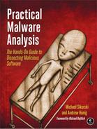
Figure 20-2 shows how the virtual function is used in Table 20-2 to determine which code to call. The first 4 bytes of the object are a pointer to the vtable. The first 4-byte entry of the vtable is a pointer to the code for the first virtual function.

Figure 20-2. C++ object with a virtual function table (vtable)

To figure out which function is being called, you find where the vtable is being accessed, and you see which offset is being called. In Table 20-2, we see the first vtable entry being accessed. To find the code that is called, we must find the vtable in memory and then go to the first function in the list.

Nonvirtual functions do not appear in a vtable because there is no need for them. The target for nonvirtual function calls is fixed at compile time.

Recognizing a Vtable

In order to identify the call destination, we need to determine the type of object and locate the vtable. If you can spot the new operator for the constructor (a concept described in the next section), you can typically discover the address of the vtable being accessed nearby.

The vtable looks like an array of function pointers. For example, Example 20-6 shows the vtable for a class with three virtual functions. When you see a vtable, only the first value in the table should have a cross-reference. The other elements of the table are accessed by their offset from the beginning of the table, and there are no accesses directly to items within the table.

Note

In this example, the line labeled off_4020F0 is the beginning of the vtable, but don’t confuse this with switch offset tables, covered in Chapter 6. A switch offset table would have offsets to locations that are not subroutines, labeled loc_###### instead of sub_######.

Example 20-6. A vtable in IDA Pro

004020F0 off_4020F0      dd offset sub_4010A0
004020F4                 dd offset sub_4010C0
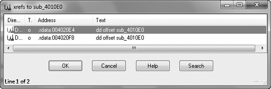
004020F8                 dd offset sub_4010E0

You can recognize virtual functions by their cross-references. Virtual functions are not directly called by other parts of the code, and when you check cross-references for a virtual function, you should not see any calls to that function. For example, Figure 20-3 shows the cross-references for a virtual function. Both cross-references are offsets to the function, and neither is a call instruction. Virtual functions almost always appear this way, whereas nonvirtual functions are typically referenced via a call instruction.

Figure 20-3. Cross-references for a virtual function

Once you have found a vtable and virtual functions, you can use that information to analyze them. When you identify a vtable, you instantly know that all functions within that table belong to the same class, and that functions within the same class are somehow related. You can also use vtables to determine if class relationships exist.

Example 20-7, an expansion of Example 20-6, includes vtables for two classes.

Example 20-7. Vtables for two different classes

004020DC off_4020DC      dd offset sub_401100
004020E0                 dd offset sub_4010C0
004020E4                ❶dd offset sub_4010E0
004020E8                 dd offset sub_401120
004020EC                 dd offset unk_402198
004020F0 off_4020F0      dd offset sub_4010A0
004020F4                 dd offset sub_4010C0
004020F8                ❷dd offset sub_4010E0

Notice that the functions at ❶ and ❷ are the same, and that there are two cross-references for this function, as shown in Figure 20-3. The two cross-references are from the two vtables that point to this function, which suggests an inheritance relationship.

Remember that child classes automatically include all functions from a parent class, unless they override it. In Example 20-7, sub_4010E0 at ❶ and ❷ is a function from the parent class that is also in the vtable for the child class, because it can also be called for the child class.

You can’t always differentiate a child class from a parent class, but if one vtable is larger than the other, it is the subclass. In this example, the vtable at offset 4020F0 is the parent class, and the vtable at offset 4020DC is the child class because its vtable is larger. (Remember that child classes always have the same functions as the parent class and may have additional functions.)

Previous Chapter

Object-Oriented Programming

Next Chapter

Creating and Destroying Objects

Table of Contents for Practical Malware Analysis

Virtual vs. Nonvirtual Functions

Use of Vtables

Recognizing a Vtable

Note

Table of Contents for
Practical Malware Analysis