Manual Unpacking

Sometimes, packed malware can be unpacked automatically by an existing program, but more often it must be unpacked manually. Manual unpacking can sometimes be done quickly, with minimal effort; other times it can be a long, arduous process.

There are two common approaches to manually unpacking a program:

Discover the packing algorithm and write a program to run it in reverse. By running the algorithm in reverse, the program undoes each of the steps of the packing program. There are automated tools that do this, but this approach is still inefficient, since the program written to unpack the malware will be specific to the individual packing program used. So, even with automation, this process takes a significant amount of time to complete.
Run the packed program so that the unpacking stub does the work for you, and then dump the process out of memory, and manually fix up the PE header so that the program is complete. This is the more efficient approach.

Let’s walk through a simple manual unpacking process. For the purposes of this example, we’ll unpack an executable that was packed with UPX. Although UPX can easily be unpacked automatically with the UPX program, it is simple and makes a good example. You’ll work through this process yourself in the first lab for this chapter.

Begin by loading the packed executable into OllyDbg. The first step is to find the OEP, which was the first instruction of the program before it was packed. Finding the OEP for a function can be one of the more difficult tasks in the manual unpacking process, and will be covered in detail later in the chapter. For this example, we will use an automated tool that is a part of the OllyDump plug-in for OllyDbg.

Note

OllyDump, a plug-in for OllyDbg, has two good features for unpacking: It can dump the memory of the current process, and it can search for the OEP for a packed executable.

In OllyDbg, select Plugins ▶ OllyDump ▶ Find OEP by Section Hop. The program will hit a breakpoint just before the OEP executes.

When that breakpoint is hit, all of the code is unpacked into memory, and the original program is ready to be run, so the code is visible and available for analysis. The only remaining step is to modify the PE header for this code so that our analysis tools can interpret the code properly.

The debugger will be broken on the instruction that is the OEP. Write down the value of the OEP, and do not close OllyDbg.

Now we’ll use the OllyDump plug-in to dump the executable. Select Plugins ▶ OllyDump ▶ Dump Debugged Process. This will dump everything from process memory onto disk. There are a few options on the screen for dumping the file to disk.

If OllyDbg just dumped the program without making any changes, then the dumped program will include the PE header of the packed program, which is not the same as the PE header of the unpacked program. We would need to change two things to correct the header:

The import table must be reconstructed.
The entry point in the PE header must point to the OEP.

Fortunately, if you don’t change any of the options on the dump screen, OllyDump will perform these steps automatically. The entry point of the executable will be set to the current instruction pointer, which in this case was the OEP, and the import table will be rebuilt. Click the Dump button, and you are finished unpacking this executable. We were able to unpack this program in just a few simple steps because OEP was located and the import table was reconstructed automatically by OllyDump. With complex unpackers it will not be so simple and the rest of the chapter covers how to unpack when OllyDump fails.

Rebuilding the Import Table with Import Reconstructor

Rebuilding the import table is complicated, and it doesn’t always work in OllyDump. The unpacking stub must resolve the imports to allow the application to run, but it does not need to rebuild the original import table. When OllyDbg fails, it’s useful to try to use Import Reconstructor (ImpRec) to perform these steps.

ImpRec can be used to repair the import table for packed programs. Run ImpRec, and open the drop-down menu at the top of the screen. You should see the running processes. Select the packed executable. Next, enter the RVA value of the OEP (not the entire address) in the OEP field on the right. For example, if the image base is 0x400000 and the OEP is 0x403904, enter 0x3904. Next, click the IAT autosearch button. You should see a window with a message stating that ImpRec found the original import address table (IAT). Now click GetImports. A listing of all the files with imported functions should appear on the left side of the main window. If the operation was successful, all the imports should say valid:YES. If the GetImports function was not successful, then the import table cannot be fixed automatically using ImpRec.

Strategies for manually fixing the table are discussed later in this chapter. For now, we’ll assume that the import table was discovered successfully. Click the Fix Dump button. You’ll be asked for the path to the file that you dumped earlier with OllyDump, and ImpRec will write out a new file with an underscore appended to the filename.

You can execute the file to make sure that everything has worked, if you’re not sure whether you’ve done it correctly. This basic unpacking process will work for most packed executables, and should be tried first.

As mentioned earlier, the biggest challenge of manually unpacking malware is finding the OEP, as we’ll discuss next.

Finding the OEP

There are many strategies for locating the OEP, and no single strategy will work against all packers. Analysts generally develop personal preferences, and they will try their favorite strategies first. But to be successful, analysts must be familiar with many techniques in case their favorite method does not work. Choosing the wrong technique can be frustrating and time-consuming. Finding the OEP is a skill that must be developed with practice. This section contains a variety of strategies to help you develop your skills, but the only way to really learn is to practice.

In order to find the OEP, you need to run the malicious program in a debugger and use single-stepping and breakpoints. Recall the different types of breakpoints described in Chapter 8. OllyDbg offers four types of breakpoints, which are triggered by different conditions: the standard INT 3 breakpoints, the memory breakpoint provided by OllyDbg, hardware breakpoints, and run tracing with break conditions.

Packed code and the unpacking stub are often unlike the code that debuggers ordinarily deal with. Packed code is often self-modifying, containing call instructions that do not return, code that is not marked as code, and other oddities. These features can confuse the debuggers and cause breakpoints to fail.

Using an automated tool to find the OEP is the easiest strategy, but much like the automated unpacking approach, these tools do not always work. You may need to find the OEP manually.

Using Automated Tools to Find the OEP

In the previous example, we used an automated tool to find the OEP. The most commonly used automatic tool for finding the OEP is the OllyDump plug-in within OllyDbg, called Find OEP by Section Hop. Normally, the unpacking stub is in one section and the executable is packed into another section. OllyDbg detects when there is a transfer from one section to another and breaks there, using either the step-over or step-into method. The step-over method will step-over any call instructions. Calls are often used to execute code in another section, and this method is designed to prevent OllyDbg from incorrectly labeling those calls the OEP. However, if a call function does not return, then OllyDbg will not locate the OEP.

Malicious packers often include call functions that do not return in an effort to confuse the analyst and the debugger. The step-into option steps into each call function, so it’s more likely to find the OEP, but also more likely to produce false positives. In practice you should try both the step-over and the step-into methods.

Finding the OEP Manually

When automated methods for finding the OEP fail, you will need to find it manually. The simplest manual strategy is to look for the tail jump. As mentioned earlier, this instruction jumps from the unpacking stub to the OEP. Normally, it’s a jmp instruction, but some malware authors make it a ret instruction in order to evade detection.

Often, the tail jump is the last valid instruction before a bunch of bytes that are invalid instructions. These bytes are padding to ensure that the section is properly byte-aligned. Generally, IDA Pro is used to search through the packed executable for the tail jump. Example 18-1 shows a simple tail jump example.

Example 18-1. A simple tail jump

00416C31   PUSH EDI
00416C32   CALL EBP
00416C34   POP EAX
00416C35   POPAD
00416C36   LEA EAX,DWORD PTR SS:[ESP-80]
00416C3A   PUSH 0
00416C3C   CMP ESP,EAX
00416C3E   JNZ SHORT Sample84.00416C3A
00416C40   SUB ESP,-80
00416C43  ❶JMP Sample84.00401000
00416C48   DB 00
00416C49   DB 00
00416C4A   DB 00
00416C4B   DB 00
00416C4C   DB 00
00416C4D   DB 00
00416C4E   DB 00

This example shows the tail jump for UPX at ❶, which is located at address 0x00416C43. Two features indicate clearly that this is the tail jump: It’s located at the end of the code, and it links to an address that is very far away. If we were examining this jump in a debugger, we would see that there are hundreds of 0x00 bytes after the jump, which is uncommon; a return generally follows a jump, but this one isn’t followed by any meaningful code.

The other feature that makes this jump stick out is its size. Normally, jumps are used for conditional statements and loops, and go to addresses that are within a few hundred bytes, but this jump goes to an address that’s 0x15C43 bytes away. That is not consistent with a reasonable jmp statement.

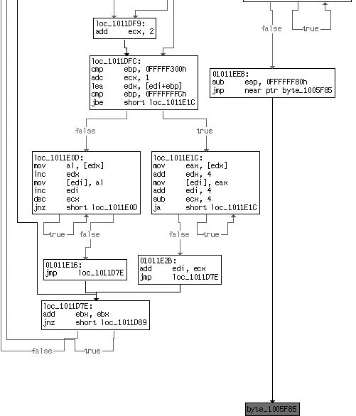
The graph view in IDA Pro often makes the tail jump very easy to spot, as shown in Figure 18-5. IDA Pro colors a jump red when it can’t determine where the jump goes. Normally, jumps are within the same function, and IDA Pro will draw an arrow to the target of a jmp instruction. In the case of a tail jump, IDA Pro encounters an error and colors the jump red.

Figure 18-5. A tail jump is highlighted in red in the IDA Pro graph view.

The tail jump transfers execution to the original program, which is packed on disk. Therefore, the tail jump goes to an address that does not contain valid instructions when the unpacking stub starts, but does contain valid instructions when the program is running. Example 18-2 shows the disassembly at the address of the jump target when the program is loaded in OllyDbg. The instruction ADD BYTE PTR DS:[EAX],AL corresponds to two 0x00 bytes, which is not a valid instruction, but OllyDbg is attempting to disassemble this instruction anyway.

Example 18-2. Instruction bytes stored at OEP before the original program is unpacked

00401000   ADD BYTE PTR DS:[EAX],AL
00401002   ADD BYTE PTR DS:[EAX],AL
00401004   ADD BYTE PTR DS:[EAX],AL
00401006   ADD BYTE PTR DS:[EAX],AL
00401008   ADD BYTE PTR DS:[EAX],AL
0040100A   ADD BYTE PTR DS:[EAX],AL
0040100C   ADD BYTE PTR DS:[EAX],AL
0040100E   ADD BYTE PTR DS:[EAX],AL

Example 18-3 contains the disassembly found at the same address when the tail jump is executed. The original executable has been unpacked, and there are now valid instructions at that location. This change is another hallmark of a tail jump.

Example 18-3. Instruction bytes stored at OEP after the original program is unpacked

00401000   CALL Sample84.004010DC
00401005   TEST EAX,EAX
00401007   JNZ SHORT Sample84.0040100E
00401009   CALL Sample84.00401018
0040100E   PUSH EAX
0040100F   CALL DWORD PTR DS:[414304] ; kernel32.ExitProcess
00401015   RETN

Another way to find the tail jump is to set a read breakpoint on the stack. Remember for read breakpoints, you must use either a hardware breakpoint or an OllyDbg memory breakpoint. Most functions in disassembly, including the unpacking stub, begin with a push instruction of some sort, which you can use to your advantage. First, make a note of the memory address on the stack where the first value is pushed, and then set a breakpoint on read for that stack location.

After that initial push, everything else on the stack will be higher on the stack (at a lower memory address). Only when the unpacking stub is complete will that stack address from the original push be accessed. Therefore, that address will be accessed via a pop instruction, which will hit the breakpoint and break execution. The tail jump is generally just after the pop instruction. It’s often necessary to try several different types of breakpoints on that address. A hardware breakpoint on read is a good type to try first. Note that the OllyDbg interface does not allow you to set a breakpoint in the stack window. You must view the stack address in the memory dump window and set a breakpoint on it there.

Another strategy for manually finding OEP is to set breakpoints after every loop in the code. This allows you to monitor each instruction being executed without consuming a huge amount of time going through the same code in a loop over and over again. Normally, the code will have several loops, including loops within loops. Identify the loops by scanning through the code and setting a breakpoint after each loop. This method is manually intensive and generally takes longer than other methods, but it is easy to comprehend. The biggest pitfall with this method is setting a breakpoint in the wrong place, which will cause the executable to run to completion without hitting the breakpoint. If this happens, don’t be discouraged. Go back to where you left off and keeping setting breakpoints further along in the process until you find the OEP.

Another common pitfall is stepping over a function call that never returns. When you step-over the function call, the program will continue to run, and the breakpoint will never be hit. The only way to address this is to start over, return to the same function call, and step-into the function instead of stepping over it. Stepping into every function can be time consuming, so it’s advisable to use trial and error to determine when to step-over versus step-into.

Another strategy for finding the tail jump is to set a breakpoint on GetProcAddress. Most unpackers will use GetProcAddress to resolve the imports for the original function. A breakpoint that hits on GetProcAddress is far into the unpacking stub, but there is still a lot of code before the tail jump. Setting a breakpoint at GetProcAddress allows you to bypass the beginning of the unpacking stub, which often contains the most complicated code.

Another approach is to set a breakpoint on a function that you know will be called by the original program and work backward. For example, in most Windows programs, the OEP can be found at the beginning of a standard wrapper of code that is outside the main method. Because the wrapper is always the same, you can find it by setting a breakpoint on one of the functions it calls.

For command-line programs, this wrapper calls the GetVersion and GetCommandLineA functions very early in the process, so you can try to break when those functions are called. The program isn’t loaded yet, so you can’t set a breakpoint on the call to GetVersion, but you can set one on the first instruction of GetVersion, which works just as well.

In GUI programs, GetModuleHandleA is usually the first function to be called. After the program breaks, examine the previous stack frame to see where the call originated. There’s a good chance that the beginning of the function that called GetModuleHandleA or GetVersion is the OEP. Beginning at the call instruction, scroll up and search for the start of the function. Most functions start with push ebp, followed by mov ebp, esp. Try to dump the program with the beginning of that function as the OEP. If you’re right, and that function is the OEP, then you are finished. If you’re wrong, then the program will still be dumped, because the unpacking stub has already finished. You will be able to view and navigate the program in IDA Pro, but you won’t necessarily know where the program starts. You might get lucky and IDA Pro might automatically identify WinMain or DllMain.

The last tactic for locating the OEP is to use the Run Trace option in OllyDbg. Run Trace gives you a number of additional breakpoint options, and allows you to set a breakpoint on a large range of addresses. For example, many packers leave the .text section for the original file. Generally, there is nothing in the .text section on disk, but the section is left in the PE header so that the loader will create space for it in memory. The OEP is always within the original .text section, and it is often the first instruction called within that section. The Run Trace option allows you to set a breakpoint to trigger whenever any instruction is executed within the .text section. When the breakpoint is triggered, the OEP can usually be found.

Repairing the Import Table Manually

OllyDump and ImpRec are usually able to rebuild the import table by searching through the program in memory for what looks like a list of imported functions. But sometimes this fails, and you need to learn a little more about how the import table works in order to analyze the malware.

The import table is actually two tables in memory. The first table is the list of names or ordinals used by the loader or unpacking stub to determine which functions are needed. The second table is the list of the addresses of all the functions that are imported. When the code is running, only the second table is needed, so a packer can remove the list of names to thwart analysis. If the list of names is removed, then you may need to manually rebuild the table.

Analyzing malware without import information is extremely difficult, so it’s best to repair the import information whenever possible. The simplest strategy is to repair the imports one at a time as you encounter them in the disassembly. To do this, open the file in IDA Pro without any import information. When you see a call to an imported function, label that imported function in the disassembly. Calls to imported functions are an indirect call to an address that is outside the loaded program, as shown in Example 18-4.

Example 18-4. Call to an imported function when the import table is not properly reconstructed

push eax
call dword_401244
...
dword_401244: 0x7c4586c8

The listing shows a call instruction with a target based on a DWORD pointer. In IDA Pro, we navigate to the DWORD and see that it has a value of 0x7c4586c8, which is outside our loaded program. Next, we open OllyDbg and navigate to the address 0x7c4586c8 to see what is there. OllyDbg has labeled that address WriteFile, and we can now label that import address as imp_WriteFile, so that we know what the function does. You’ll need to go through these steps for each import you encounter. The cross-referencing feature of IDA Pro will then label all calls to the imported functions. Once you’ve labeled enough functions, you can effectively analyze the malware.

The main drawbacks to this method are that you may need to label a lot of functions, and you cannot search for calls to an import until you have labeled it. The other drawback to this approach is that you can’t actually run your unpacked program. This isn’t a showstopper, because you can use the unpacked program for static analysis, and you can still use the packed program for dynamic analysis.

Another strategy, which does allow you to run the unpacked program, is to manually rebuild the import table. If you can find the table of imported functions, then you can rebuild the original import table by hand. The PE file format is an open standard, and you can enter the imported functions one at time, or you could write a script to enter the information for you. The biggest drawback is that this approach can be very tedious and time-consuming.

Note

Sometimes malware authors use more than one packer. This doubles the work for the analyst, but with persistence, it’s usually possible to unpack even double-packed malware. The strategy is simple: Undo the first layer of packing using any of the techniques we’ve just described, and then repeat to undo the second layer of packing. The strategies are the same, regardless of the number of packers used.

Previous Chapter

Automated Unpacking

Next Chapter

Tips and Tricks for Common Packers

Table of Contents for Practical Malware Analysis

Manual Unpacking

Note

Rebuilding the Import Table with Import Reconstructor

Finding the OEP

Using Automated Tools to Find the OEP

Finding the OEP Manually

Repairing the Import Table Manually

Note

Table of Contents for
Practical Malware Analysis