The simplest thing you can do with a debugger is to single-step through a program, which means that you run a single instruction and then return control to the debugger. Single-stepping allows you to see everything going on within a program.

It is possible to single-step through an entire program, but you should not do it for complex programs because it can take such a long time. Single-stepping is a good tool for understanding the details of a section of code, but you must be selective about which code to analyze. Focus on the big picture, or you’ll get lost in the details.

For example, the disassembly in Example 8-1 shows how you might use a debugger to help understand a section of code.

mov     edi, DWORD_00406904
mov     ecx, 0x0d
LOC_040106B2
xor     [edi], 0x9C
inc     edi
loopw   LOC_040106B2
...
DWORD:00406904:   F8FDF3D0❶

The listing shows a data address accessed and modified in a loop. The data value shown at the end ❶ doesn’t appear to be ASCII text or any other recognizable value, but you can use a debugger to step through this loop to reveal what this code is doing.

If we were to single-step through this loop with either WinDbg or OllyDbg, we would see the data being modified. For example, in Example 8-2, you see the 13 bytes modified by this function changing each time through the loop. (This listing shows the bytes at those addresses along with their ASCII representation.)

D0F3FDF8 D0F5FEEE FDEEE5DD 9C (.............)
4CF3FDF8 D0F5FEEE FDEEE5DD 9C (L............)
4C6FFDF8 D0F5FEEE FDEEE5DD 9C (Lo...........)
4C6F61F8 D0F5FEEE FDEEE5DD 9C (Loa..........)
. . . SNIP . . .
4C6F6164 4C696272 61727941 00 (LoadLibraryA.)

With a debugger attached, it is clear that this function is using a single-byte XOR function to decode the string LoadLibraryA. It would have been more difficult to identify that string with only static analysis.

When single-stepping through code, the debugger stops after every instruction. However, while you are generally concerned with what a program is doing, you may not be concerned with the functionality of each call. For example, if your program calls LoadLibrary, you probably don’t want to step through every instruction of the LoadLibrary function.

To control the instructions that you see in your debugger, you can step-over or step-into instructions. When you step-over call instructions, you bypass them. For example, if you step-over a call, the next instruction you will see in your debugger will be the instruction after the function call returns. If, on the other hand, you step-into a call instruction, the next instruction you will see in the debugger is the first instruction of the called function.

Stepping-over allows you to significantly decrease the amount of instructions you need to analyze, at the risk of missing important functionality if you step-over the wrong functions. Additionally, certain function calls never return, and if your program calls a function that never returns and you step-over it, the debugger will never regain control. When this happens (and it probably will), restart the program and step to the same location, but this time, step-into the function.

When stepping-into a function, it is easy to quickly begin single-stepping through instructions that have nothing to with what you are analyzing. When analyzing a function, you can step-into a function that it calls, but then it will call another function, and then another. Before long, you are analyzing code that has little or no relevance to what you are seeking. Fortunately, most debuggers will allow you to return to the calling function, and some debuggers have a step-out function that will run until after the function returns. Other debuggers have a similar feature that executes until a return instruction immediately prior to the end of the function.

Breakpoints are used to pause execution and allow you to examine a program’s state. When a program is paused at a breakpoint, it is referred to as broken. Breakpoints are needed because you can’t access registers or memory addresses while a program is running, since these values are constantly changing.

Example 8-3 demonstrates where a breakpoint would be useful. In this example, there is a call to EAX. While a disassembler couldn’t tell you which function is being called, you could set a breakpoint on that instruction to find out. When the program hits the breakpoint, it will be stopped, and the debugger will show you the value of EAX, which is the destination of the function being called.

00401008   mov     ecx, [ebp+arg_0]
0040100B   mov     eax, [edx]
0040100D   call    eax

Another example in Example 8-4 shows the beginning of a function with a call to CreateFile to open a handle to a file. In the assembly, it is difficult to determine the name of the file, although part of the name is passed in as a parameter to the function. To find the file in disassembly, you could use IDA Pro to search for all the times that this function is called in order to see which arguments are passed, but those values could in turn be passed in as parameters or derived from other function calls. It could very quickly become difficult to determine the filename. Using a debugger makes this task very easy.

0040100B  xor     eax, esp
0040100D  mov     [esp+0D0h+var_4], eax
00401014  mov     eax, edx
00401016  mov     [esp+0D0h+NumberOfBytesWritten], 0
0040101D  add     eax, 0FFFFFFFEh
00401020  mov     cx, [eax+2]
00401024  add     eax, 2
00401027  test    cx, cx
0040102A  jnz     short loc_401020
0040102C  mov     ecx, dword ptr ds:a_txt ; ".txt"
00401032  push    0               ; hTemplateFile
00401034  push    0               ; dwFlagsAndAttributes
00401036  push    2               ; dwCreationDisposition
00401038  mov     [eax], ecx
0040103A  mov     ecx, dword ptr ds:a_txt+4
00401040  push    0               ; lpSecurityAttributes
00401042  push    0               ; dwShareMode
00401044  mov     [eax+4], ecx
00401047  mov     cx, word ptr ds:a_txt+8
0040104E  push    0               ; dwDesiredAccess
00401050  push    edx             ; lpFileName
00401051  mov     [eax+8], cx
00401055 ❶call    CreateFileW ; CreateFileW(x,x,x,x,x,x,x)

We set a breakpoint on the call to CreateFileW at ❶, and then look at the values on the stack when the breakpoint is triggered. Figure 8-1 shows a screenshot of the same instruction at a breakpoint within the WinDbg debugger. After the breakpoint, we display the first parameter to the function as an ASCII string using WinDbg. (You’ll learn how to do this in Chapter 10, which covers WinDbg.)

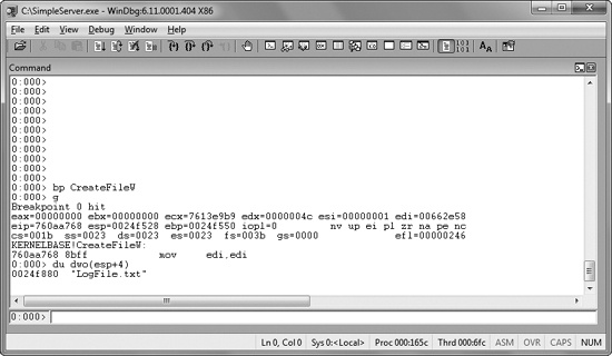
Figure 8-1. Using a breakpoint to see the parameters to a function call. We set a breakpoint on CreateFileW and then examine the first parameter of the stack.

In this case, it is clear that the file being created is called LogFile.txt. While we could have figured this out with IDA Pro, it was faster and easier to get the information with a debugger.

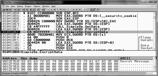
Now imagine that we have a piece of malware and a packet capture. In the packet capture, we see encrypted data. We can find the call to send, and we discover the encryption code, but it is difficult to decrypt the data ourselves, because we don’t know the encryption routine or key. Luckily, we can use a debugger to simplify this task because encryption routines are often separate functions that transform the data.

If we can find where the encryption routine is called, we can set a breakpoint before the data is encrypted and view the data being sent, as shown in the disassembly for this function at ❶ in Example 8-5.

004010D0  sub     esp, 0CCh
004010D6  mov     eax, dword_403000
004010DB  xor     eax, esp
004010DD  mov     [esp+0CCh+var_4], eax
004010E4  lea     eax, [esp+0CCh+buf]
004010E7  call    GetData
004010EC  lea     eax, [esp+0CCh+buf]
004010EF ❶call    EncryptData
004010F4  mov     ecx, s
004010FA  push    0               ; flags
004010FC  push    0C8h            ; len
00401101  lea     eax, [esp+0D4h+buf]
00401105  push    eax             ; buf
00401106  push    ecx             ; s
00401107  call    ds:Send

Figure 8-2 shows a debug window from OllyDbg that displays the buffer in memory prior to being sent to the encryption routine. The top window shows the instruction with the breakpoint, and the bottom window displays the message. In this case, the data being sent is Secret Message, as shown in the ASCII column at the bottom right.

Figure 8-2. Viewing program data prior to the encryption function call

You can use several different types of breakpoints, including software execution, hardware execution, and conditional breakpoints. Although all breakpoints serve the same general purpose, depending on the situation, certain breakpoints will not work where others will. Let’s look at how each one works.

00401130 55                ❶push    ebp
00401131 8B EC              mov     ebp, esp
00401133 83 E4 F8           and     esp, 0FFFFFFF8h
00401136 81 EC A4 03 00 00  sub     esp, 3A4h
0040113C A1 00 30 40 00     mov     eax, dword_403000

00401130 ❷CC 8B EC 83
00401134  E4 F8 81 EC
00401138  A4 03 00 00
0040113C  A1 00 30 40
00401140  00