Common Cryptographic Algorithms

Simple cipher schemes that are the equivalent of substitution ciphers differ greatly from modern cryptographic ciphers. Modern cryptography takes into account the exponentially increasing computing capabilities, and ensures that algorithms are designed to require so much computational power that breaking the cryptography is impractical.

The simple cipher schemes we have discussed previously don’t even pretend to be protected from brute-force measures. Their main purpose is to obscure. Cryptography has evolved and developed over time, and it is now integrated into every aspect of computer use, such as SSL in a web browser or the encryption used at a wireless access point. Why then, does malware not always take advantage of this cryptography for hiding its sensitive information?

Malware often uses simple cipher schemes because they are easy and often sufficient. Also, using standard cryptography does have potential drawbacks, particularly with regard to malware:

Cryptographic libraries can be large, so malware may need to statically integrate the code or link to existing code.
Having to link to code that exists on the host may reduce portability.
Standard cryptographic libraries are easily detected (via function imports, function matching, or the identification of cryptographic constants).
Users of symmetric encryption algorithms need to worry about how to hide the key.

Many standard cryptographic algorithms rely on a strong key to store their secrets. The idea is that the algorithm itself is widely known, but without the key, it is nearly impossible (that is, it would require a massive amount of work) to decrypt the cipher text. In order to ensure a sufficient amount of work for decrypting, the key must typically be long enough so that all of the potential keys cannot be easily tested. For the standard algorithms that malware might use, the trick is to identify not only the algorithm, but also the key.

There are several easy ways to identify the use of standard cryptography. They include looking for strings and imports that reference cryptographic functions and using several tools to search for specific content.

Recognizing Strings and Imports

One way to identify standard cryptographic algorithms is by recognizing strings that refer to the use of cryptography. This can occur when cryptographic libraries such as OpenSSL are statically compiled into malware. For example, the following is a selection of strings taken from a piece of malware compiled with OpenSSL encryption:

OpenSSL 1.0.0a
SSLv3 part of OpenSSL 1.0.0a
TLSv1 part of OpenSSL 1.0.0a
SSLv2 part of OpenSSL 1.0.0a
You need to read the OpenSSL FAQ, http://www.openssl.org/support/faq.html
%s(%d): OpenSSL internal error, assertion failed: %s
AES for x86, CRYPTOGAMS by <appro@openssl.org>

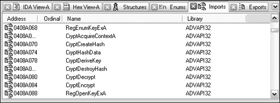
Another way to look for standard cryptography is to identify imports that reference cryptographic functions. For example, Figure 13-9 is a screenshot from IDA Pro showing some cryptographic imports that provide services related to hashing, key generation, and encryption. Most (though not all) of the Microsoft functions that pertain to cryptography start with Crypt, CP (for Cryptographic Provider), or Cert.

Figure 13-9. IDA Pro imports listing showing cryptographic functions

Searching for Cryptographic Constants

A third basic method of detecting cryptography is to use a tool that can search for commonly used cryptographic constants. Here, we’ll look at using IDA Pro’s FindCrypt2 and Krypto ANALyzer.

Using FindCrypt2

IDA Pro has a plug-in called FindCrypt2, included in the IDA Pro SDK (or available from http://www.hex-rays.com/idapro/freefiles/findcrypt.zip), which searches the program body for any of the constants known to be associated with cryptographic algorithms. This works well, since most cryptographic algorithms employ some type of magic constant. A magic constant is some fixed string of bits that is associated with the essential structure of the algorithm.

Note

Some cryptographic algorithms do not employ a magic constant. Notably, the International Data Encryption Algorithm (IDEA) and the RC4 algorithm build their structures on the fly, and thus are not in the list of algorithms that will be identified. Malware often employs the RC4 algorithm, probably because it is small and easy to implement in software, and it has no cryptographic constants to give it away.

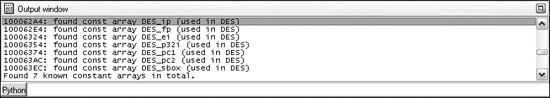
FindCrypt2 runs automatically on any new analysis, or it can be run manually from the plug-in menu. Figure 13-10 shows the IDA Pro output window with the results of running FindCrypt2 on a malicious DLL. As you can see, the malware contains a number of constants that begin with DES. By identifying the functions that reference these constants, you can quickly get a handle on the functions that implement the cryptography.

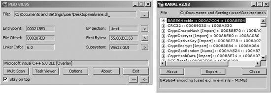
Figure 13-10. IDA Pro FindCrypt2 output

Using Krypto ANALyzer

A tool that uses the same principles as the FindCrypt2 IDA Pro plug-in is the Krypto ANALyzer (KANAL). KANAL is a plug-in for PEiD (http://www.peid.has.it/) and has a wider range of constants (though as a result, it may tend to produce more false positives). In addition to constants, KANAL also recognizes Base64 tables and cryptography-related function imports.

Figure 13-11 shows the PEiD window on the left and the KANAL plug-in window on the right. PEiD plug-ins can be run by clicking the arrow in the lower-right corner. When KANAL is run, it identifies constants, tables, and cryptography-related function imports in a list. Figure 13-11 shows KANAL finding a Base64 table, a CRC32 constant, and several Crypt... import functions in malware.

Figure 13-11. PEiD and Krypto ANALyzer (KANAL) output

Searching for High-Entropy Content

Another way to identify the use of cryptography is to search for high-entropy content. In addition to potentially highlighting cryptographic constants or cryptographic keys, this technique can also identify encrypted content itself. Because of the broad reach of this technique, it is potentially applicable in cases where cryptographic constants are not found (like RC4).

Warning

The high-entropy content technique is fairly blunt and may best be used as a last resort. Many types of content—such as pictures, movies, audio files, and other compressed data—display high entropy and are indistinguishable from encrypted content except for their headers.

The IDA Entropy Plugin (http://www.smokedchicken.org/2010/06/ida-entropy-plugin.html) is one tool that implements this technique for PE files. You can load the plug-in into IDA Pro by placing the ida-ent.plw file in the IDA Pro plug-ins directory.

Let’s use as our test case the same malware that showed signs of DES encryption from Figure 13-10. Once the file is loaded in IDA Pro, start the IDA Entropy Plugin. The initial window is the Entropy Calculator, which is shown as the left window in Figure 13-12. Any segment can be selected and analyzed individually. In this case, we are focused on a small portion of the rdata segment. The Deep Analyze button uses the parameters specified (chunk size, step size, and maximum entropy) and scans the specified area for chunks that exceed the listed entropy. If you compare the output in Figure 13-10 with the results returned in the deep analysis results window in Figure 13-12, you will see that the same addresses around 0x100062A4 are highlighted. The IDA Pro Entropy Plugin has found the DES constants (which indicates a high degree of entropy) with no knowledge of the constants themselves!

Figure 13-12. IDA Pro Entropy Plugin

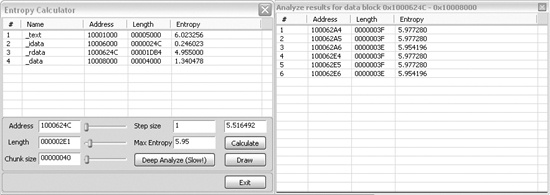
In order to use entropy testing effectively, it is important to understand the dependency between the chunk size and entropy score. The setting shown in Figure 13-12 (chunk size of 64 with maximum entropy of 5.95) is actually a good generic test that will find many types of constants, and will actually locate any Base64-encoding string as well (even ones that are nonstandard).

A 64-byte string with 64 distinct byte values has the highest possible entropy value. The 64 values are related to the entropy value of 6 (which refers to 6 bits of entropy), since the number of values that can be expressed with 6 bits is 64.

Another setting that can be useful is a chunk size of 256 with entropy above 7.9. This means that there is a string of 256 consecutive bytes, reflecting nearly all 256 possible byte values.

The IDA Pro Entropy Plugin also has a tool that provides a graphical overview of the area of interest, which can be used to guide the values you should select for the maximum entropy score, and also helps to determine where to focus. The Draw button produces a graph that shows higher-entropy regions as lighter bars and lower-entropy regions as darker bars. By hovering over the graph with the mouse cursor, you can see the raw entropy scores for that specific spot on the graph. Because the entropy map is difficult to appreciate in printed form, a line graph of the same file is included in Figure 13-13 to illustrate how the entropy map can be useful.

The graph in Figure 13-13 was generated using the same chunk size of 64. The graph shows only high values, from 4.8 to 6.2. Recall that the maximum entropy value for that chunk size is 6. Notice the spike that reaches 6 above the number 25000. This is the same area of the file that contains the DES constants highlighted in Figure 13-10 and Figure 13-12.

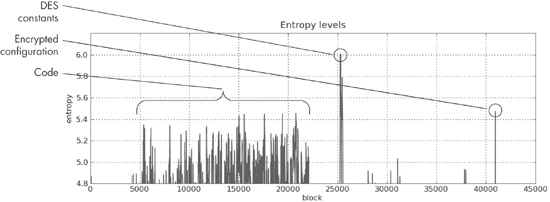
Figure 13-13. Entropy graph for a malicious executable

A couple of other features stand out. One is the plateau between blocks 4000 and 22000. This represents the actual code, and it is typical of code to reach an entropy value of this level. Code is typically contiguous, so it will form a series of connected peaks.

A more interesting feature is the spike at the end of the file to about 5.5. The fact that it is a fairly high value unconnected with any other peaks makes it stand out. When analyzed, it is found to be DES-encrypted configuration data for the malware, which hides its command-and-control information.

Table of Contents for Practical Malware Analysis