The .gpx files store all the points' details in the WGS 84 spatial reference system; therefore, we created the rk_track_points table with SRID (4326).

After creating the rk_track_points table, we imported all of the .gpx files in the runkeeper_gpx directory using a bash script. The bash script iterates all of the files with the extension *.gpx in the runkeeper_gpx directory. For each of these files, the script runs the ogr2ogr command, importing the .gpx files to PostGIS using the GPX GDAL driver (for more details, go to http://www.gdal.org/drv_gpx.html).

In the GDAL's abstraction, a .gpx file is an OGR data source composed of several layers as follows:

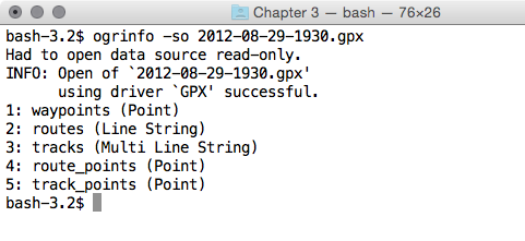
In the .gpx files (OGR data sources), you have just the tracks and track_points layers. As a shortcut, you could have imported just the tracks layer using ogr2ogr, but you would need to start from the track_points layer in order to generate the tracks layer itself, using some PostGIS functions. This is why in the ogr2ogr section in the bash script, we imported to the rk_track_points PostGIS table the point geometries from the track_points layer, plus a couple of useful attributes, such as elevation and timestamp.

Once the records were imported, we fed a new polylines table named tracks using a subquery and selected all of the point geometries and their dates and times from the rk_track_points table, grouped by date and with the geometries aggregated using the ST_MakeLine function. This function was able to create linestrings from point geometries (for more details, go to http://www.postgis.org/docs/ST_MakeLine.html).

You should not forget to sort the points in the subquery by datetime; otherwise, you will obtain an irregular linestring, jumping from one point to the other and not following the correct order.

After loading the tracks table, we tested the two spatial queries.

At first, you got a month-by-month report of the total distance run by the runner. For this purpose, you selected all of the track records grouped by date (year and month), with the total distance obtained by summing up the lengths of the single tracks (obtained with the ST_Length function). To get the year and the month from the run_date function, you used the PostgreSQL EXTRACT function. Be aware that if you measure the distance using geometries in the WGS 84 system, you will obtain it in degree units. For this reason, you have to project the geometries to a planar metric system designed for the specific region from which the data will be projected.

For large-scale areas, such as in our case where we have points that span all around Europe, as shown in the last query results, a good option is to use the geography data type introduced with PostGIS 1.5. The calculations may be slower, but are much more accurate than in other systems. This is the reason why you cast the geometries to the geography data type before making measurements.

The last spatial query used a spatial join with the ST_Intersects function to get the name of the country for each track the runner ran (with the assumption that the runner didn't run cross-border tracks). Getting the total distance run per country is just a matter of aggregating the selection on the country_name field and aggregating the track distances with the PostgreSQL SUM operator.