With preparations in place, now we are ready to create the Voronoi diagram. First, we will create the table that will contain the MultiPolygon:

DROP TABLE IF EXISTS chp04.voronoi_diagram; 
CREATE TABLE chp04.voronoi_diagram( 
  gid serial PRIMARY KEY, 
  the_geom geometry(MultiPolygon, 3734) 
);

Now, to calculate the Voronoi diagram, we use ST_Collect in order to provide a MultiPoint object for the ST_VoronoiPolygons function. The output of this alone would be a GeometryCollection; however, we are interested in getting a MultiPolygon instead, so we need to use the ST_CollectionExtract function, which when given the number 3 as the second parameter, extracts all polygons from a GeometryCollection:

INSERT INTO chp04.voronoi_diagram(the_geom)( 
  SELECT ST_CollectionExtract( 
    ST_SetSRID( 
      ST_VoronoiPolygons(points.the_geom),   
    3734), 
  3) 
  FROM ( 
    SELECT 
    ST_Collect(the_geom) as the_geom 
    FROM chp04.voronoi_test_points 
  )
as points);  

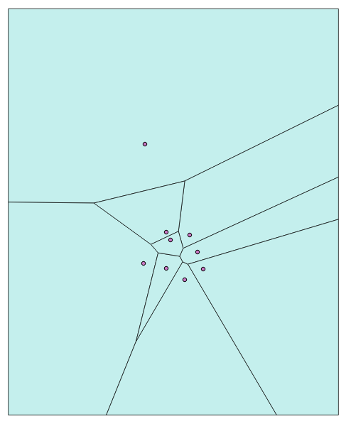
If we import the layers for voronoi_test_points and voronoi_diagram into a desktop GIS, we get the following Voronoi diagram of the randomly generated points:

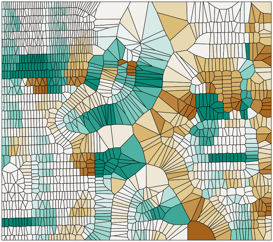
Now we can process much larger datasets. The following is a Voronoi diagram derived from the address points from the Improving proximity filtering with KNN – advanced recipe, with the coloration based on the azimuth to the nearest street, also calculated in that recipe: