Let us say that a colleague asks for the monthly minimum temperature data for San Francisco during the summer months as a single raster file. This entails restricting our PRISM rasters to June, July, and August, clipping each monthly raster to San Francisco's boundaries, creating one raster with each monthly raster as a band, and then outputting the combined raster to a portable raster format. We will convert the combined raster to the GeoTIFF format:

WITH months AS ( -- extract monthly rasters clipped to San Francisco 
   SELECT prism.month_year, ST_Union(ST_Clip(prism.rast, 2, ST_Transform(sf.geom, 4269), TRUE)) AS rast 
  FROM chp05.prism 
  JOIN chp05.sfpoly sf ON ST_Intersects(prism.rast, ST_Transform(sf.geom, 4269)) 
  WHERE prism.month_year BETWEEN '2017-06-01'::date AND '2017-08-01'::date 
  GROUP BY prism.month_year 
  ORDER BY prism.month_year 
), summer AS ( -- new raster with each monthly raster as a band 
  SELECT ST_AddBand(NULL::raster, array_agg(rast)) AS rast FROM months) 
SELECT -- export as GeoTIFF ST_AsTIFF(rast) AS content FROM summer; 

To filter our PRISM rasters, we use ST_Intersects() to keep only those raster tiles that spatially intersect San Francisco's boundaries. We also remove all rasters whose relevant month is not June, July, or August. We then use ST_AddBand() to create a new raster with each summer month's new raster band. Finally, we pass the combined raster to ST_AsTIFF() to generate a GeoTIFF.

If you output the returned value from ST_AsTIFF() to a file, run gdalinfo on that file. The gdalinfo output shows that the GeoTIFF file has three bands, and the coordinate system of SRID 4322:

Driver: GTiff/GeoTIFF
Files: surface.tif
Size is 20, 7
Coordinate System is:
GEOGCS["WGS 72",
  DATUM["WGS_1972",
  SPHEROID["WGS 72",6378135,298.2600000000045, AUTHORITY["EPSG","7043"]],
           TOWGS84[0,0,4.5,0,0,0.554,0.2263], AUTHORITY["EPSG","6322"]],
           PRIMEM["Greenwich",0], UNIT["degree",0.0174532925199433],
           AUTHORITY["EPSG","4322"]]
  Origin = (-123.145833333333314,37.937500000000114)
  Pixel Size = (0.041666666666667,-0.041666666666667)
  Metadata:
    AREA_OR_POINT=Area
  Image Structure Metadata:
    INTERLEAVE=PIXEL
Corner Coordinates:
  Upper Left  (-123.1458333,  37.9375000) (123d 8'45.00"W, 37d56'15.00"N)
  Lower Left  (-123.1458333,  37.6458333) (123d 8'45.00"W, 37d38'45.00"N)
  Upper Right (-122.3125000,  37.9375000) (122d18'45.00"W, 37d56'15.00"N)
  Lower Right (-122.3125000,  37.6458333) (122d18'45.00"W, 37d38'45.00"N)
  Center      (-122.7291667,  37.7916667) (122d43'45.00"W, 37d47'30.00"N)
Band 1 Block=20x7 Type=Float32, ColorInterp=Gray
  NoData Value=-9999
Band 2 Block=20x7 Type=Float32, ColorInterp=Undefined
  NoData Value=-9999
Band 3 Block=20x7 Type=Float32, ColorInterp=Undefined
  NoData Value=-9999

The problem with the GeoTIFF raster is that we generally can't view it in a standard image viewer. If we use ST_AsPNG() or ST_AsJPEG(), the image generated is much more readily viewable. But PNG and JPEG images are limited by the supported pixel types 8BUI and 16BUI (PNG only). Both formats are also limited to, at the most, three bands (four, if there is an alpha band).

To help get around various file format limitations, we can use ST_MapAlgebra(), ST_Reclass() , or ST_ColorMap(), for this recipe. The ST_ColorMap() function converts a raster band of any pixel type to a set of up to four 8BUI bands. This facilitates creating a grayscale, RGB, or RGBA image that is then passed to ST_AsPNG(), or ST_AsJPEG().

Taking our query for computing a slope raster of San Francisco from our SRTM raster in a prior recipe, we can apply one of ST_ColorMap() function's built-in colormaps, and then pass the resulting raster to ST_AsPNG() to create a PNG image:

WITH r AS (SELECT ST_Transform(ST_Union(srtm.rast), 3310) AS rast 
  FROM chp05.srtm 
  JOIN chp05.sfpoly sf ON ST_DWithin(ST_Transform(srtm.rast::geometry, 3310),
  ST_Transform(sf.geom, 3310), 1000) 
), cx AS ( 
  SELECT ST_AsRaster(ST_Transform(sf.geom, 3310), r.rast) AS rast 
  FROM sfpoly sf CROSS JOIN r 
) 
SELECT ST_AsPNG(ST_ColorMap(ST_Clip(ST_Slope(r.rast, 1, cx.rast), ST_Transform(sf.geom, 3310) ), 'bluered')) AS rast 
FROM r 
CROSS JOIN cx 
CROSS JOIN chp05.sfpoly sf; 

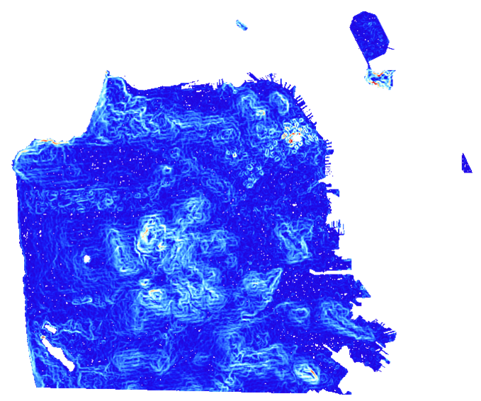
The bluered colormap sets the minimum, median, and maximum pixel values to dark blue, pale white, and bright red, respectively. Pixel values between the minimum, median, and maximum values are assigned colors that are linearly interpolated from the minimum to median or median to maximum range. The resulting image readily shows where the steepest slopes in San Francisco are.

The following is a PNG image generated by applying the bluered colormap with ST_ColorMap() and ST_AsPNG(). The pixels in red represent the steepest slopes:

In our use of ST_AsTIFF() and ST_AsPNG(), we passed the raster to be converted as the sole argument. Both of these functions have additional parameters to customize the output TIFF or PNG file. These additional parameters include various compression and data organization settings.