The steps you need to do to complete this recipe are as follows:

1. Set the PostgreSQL search_path variable such that all your newly created database objects will be stored in the chp03 schema, using the following code:

      postgis_cookbook=# SET search_path TO chp03,public; 

2. Suppose you need a less-detailed version of the states layer for your mapping website or to deploy to a client; you could consider using the ST_SimplifyPreserveTopology function as follows:

      postgis_cookbook=# CREATE TABLE states_simplify_topology AS 
        SELECT ST_SimplifyPreserveTopology(ST_Transform(
          the_geom, 2163), 500) FROM states;

3. The previous command works quickly, using a variant of the Douglas-Peucker algorithm, and effectively reduces the vertex number. But the resulting polygons, in some cases, are not adjacent any more. If you zoom in at any polygon border, you should notice something shown in the following screenshot: there are holes and overlaps along the shared border between two polygons. This is because PostGIS is using the OGC Simple Feature model, which doesn't implement topology, so the function just removes the redundant vertex without taking the adjacent polygons into consideration:

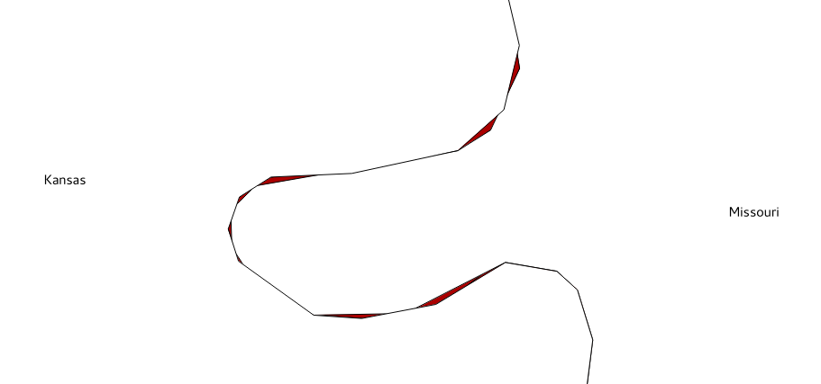
4. It looks like the ST_SimplifyPreserveTopology function, while working well with linear features, produces topological anomalies with polygons. In case you want topological simplification, another approach is the following code suggested by Paul Ramsey (http://gis.stackexchange.com/questions/178/simplifying-adjacent-polygons) and improved in a Webspaces blog post (http://webspaces.net.nz/page.php?view=polygon-dissolve-and-generalise):

      SET search_path TO chp03, public; 
      -- first project the spatial table to a planar system 
        (recommended for simplification operations) 
      CREATE TABLE states_2163 AS SELECT ST_Transform
        (the_geom, 2163)::geometry(MultiPolygon, 2163) 
        AS the_geom, state FROM states; 
      -- now decompose the geometries from multipolygons to polygons (2895) 
        using the ST_Dump function 
      CREATE TABLE polygons AS SELECT (ST_Dump(the_geom)).geom AS the_geom 
        FROM states_2163; 
      -- now decompose from polygons (2895) to rings (3150) 
        using the ST_DumpRings function 
      CREATE TABLE rings AS SELECT (ST_DumpRings(the_geom)).geom 
        AS the_geom FROM polygons; 
      -- now decompose from rings (3150) to linestrings (3150) 
        using the ST_Boundary function 
      CREATE TABLE ringlines AS SELECT(ST_boundary(the_geom)) 
        AS the_geom FROM rings; 
      -- now merge all linestrings (3150) in a single merged linestring 
        (this way duplicate linestrings at polygon borders disappear) 
      CREATE TABLE mergedringlines AS SELECT ST_Union(the_geom) 
        AS the_geom FROM ringlines; 
      -- finally simplify the linestring with a tolerance of 150 meters 
      CREATE TABLE simplified_ringlines AS SELECT 
      ST_SimplifyPreserveTopology(the_geom, 150) 
      AS the_geom FROM mergedringlines; 
      -- now compose a polygons collection from the linestring 
      using the ST_Polygonize function 
      CREATE TABLE simplified_polycollection AS SELECT 
        ST_Polygonize(the_geom) AS the_geom FROM simplified_ringlines; 
      -- here you generate polygons (2895) from the polygons collection 
        using ST_Dumps 
      CREATE TABLE simplified_polygons AS SELECT 
        ST_Transform((ST_Dump(the_geom)).geom, 
        4326)::geometry(Polygon,4326) 
        AS the_geom FROM simplified_polycollection; 
      -- time to create an index, to make next operations faster 
        CREATE INDEX simplified_polygons_gist ON simplified_polygons 
        USING GIST (the_geom); 
      -- now copy the state name attribute from old layer with a spatial 
        join using the ST_Intersects and ST_PointOnSurface function 
      CREATE TABLE simplified_polygonsattr AS SELECT new.the_geom, 
        old.state FROM simplified_polygons new, states old 
        WHERE ST_Intersects(new.the_geom, old.the_geom) 
        AND ST_Intersects(ST_PointOnSurface(new.the_geom), old.the_geom); 
      -- now make the union of all polygons with a common name 
      CREATE TABLE states_simplified AS SELECT ST_Union(the_geom) 
        AS the_geom, state FROM simplified_polygonsattr GROUP BY state;

5. This approach seems to work smoothly, but if you try to increment the simplifying tolerance from 150 to, let's say, 500 meters, you will again end up with topological anomalies (test this yourself). A better approach would be to use the PostGIS topology (you will do this in the Simplifying geometries with PostGIS topology recipe) or an external GIS tool that is able to manage topological operations the way GRASS can. For this recipe, you will use the GRASS approach.
6. Install GRASS on your system if you don't have it. Then, create a directory to contain the GRASS database (in GRASS jargon, a GISDBASE), as follows:

      $ mkdir grass_db

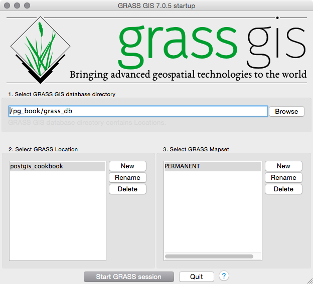
7. Now, start GRASS by typing grass in the Linux command prompt or by double-clicking on the GRASS GUI icon in Windows (Start | All Programs | OSGeo4W | GRASS GIS 6.4.3 | GRASS 6.4.3 GUI) or on Applications in macOS. You will be prompted to select the grass_db database as the GIS data directory but should instead select the one you created in the previous step.
8. Using the Location Wizard button, create a location named postgis_cookbook with the title PostGIS Cookbook (GRASS uses subdirectories named locations, where all of the data is kept in the same coordinate system, map projection, and geographical boundaries).
9. When creating the new location, select the EPSG with SRID 2163 as the spatial reference system (you need to select the Select EPSG code of spatial reference system option under Choose method for creating a new location).

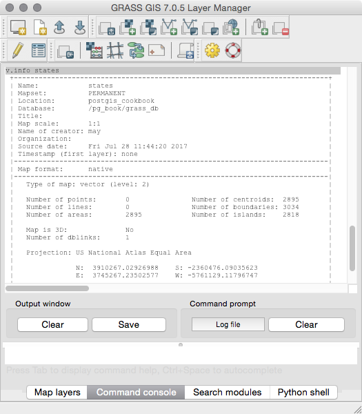
10. Now start GRASS by clicking on the Start GRASS button. The program's command line will start as shown in the following screenshot:

11. Import the states PostGIS spatial table to the GRASS location. To do so, use the v.in.ogr GRASS command, which will then use the OGR PostgreSQL driver (in fact, the PostGIS connection string syntax is the same):

      GRASS 6.4.1 (postgis_cookbook):~ > v.in.ogr 
      input=PG:"dbname='postgis_cookbook' user='me' 
      password='mypassword'" layer=chp03.states_2163 out=states

12. GRASS will import the OGR PostGIS table and simultaneously build the topology for this layer, which is composed of points, lines, areas, and so on. The v.info command can be used in combination with the -c option to check the attributes table and get more information on the imported layer, as follows:

      GRASS 6.4.1 (postgis_cookbook):~ > v.info states

13. Now, you can simplify the polygon geometries using the v.generalizeGRASS command with a tolerance (threshold) of 500 meters. If you are using the same dataset used in this recipe, you will end up with 47,191 vertices from the original 346,914 vertices, composing 1,919 polygons (areas) from the original 2,895 polygons:

      GRASS 6.4.1 (postgis_cookbook):~ > v.generalize input=states 
      output=states_generalized_from_grass method=douglas threshold=500

14. Export the results back to PostGIS using the v.out.ogr command (the v.in.ogr counterpart) as follows:

      GRASS 6.4.1 (postgis_cookbook):~ > v.out.ogr 
      input=states_generalized_from_grass 
      type=area dsn=PG:"dbname='postgis_cookbook' user='me' 
      password='mypassword'" olayer=chp03.states_simplified_from_grass 
      format=PostgreSQL

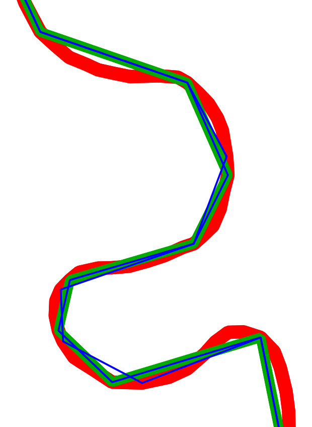
15. Now, open a desktop GIS and check for differences between the geometry simplification performed by the ST_SimplifyPreserveTopology PostGIS function and GRASS. There should be no holes or overlaps at shared polygon borders. In the following screenshot, the original layer boundaries are in red, the boundaries built by ST_SimplifyPreserveTopology are in blue, and those built by GRASS are in green: