PostGIS includes the raster_columns view to provide a high-level summary of all the raster columns found in the database. This view is similar to the geometry_columns and geography_columns views in function and form.

Let's run the following SQL query in the raster_columns view to see what information is available in the prism table:

SELECT 
  r_table_name, 
  r_raster_column, 
  srid, 
  scale_x, 
  scale_y, 
  blocksize_x, 
  blocksize_y, 
  same_alignment, 
  regular_blocking, 
  num_bands, 
  pixel_types, 
  nodata_values, 
  out_db, 
  ST_AsText(extent) AS extent FROM raster_columns WHERE r_table_name = 'prism'; 

The SQL query returns a record similar to the following:

(1 row)

If you look back at the gdalinfo output for one of the PRISM rasters, you'll see that the values for the scales (the pixel size) match. The flags passed to raster2pgsql, specifying tile size and SRID, worked.

Let's see what the metadata of a single raster tile looks like. We will use the ST_Metadata() function:

SELECT  rid,  (ST_Metadata(rast)).* 
FROM chp05.prism 
WHERE month_year = '2017-03-01'::date 
LIMIT 1; 

The output will look similar to the following:

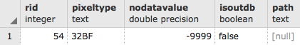
Use ST_BandMetadata() to examine the first and only band of raster tiles at the record ID 54:

SELECT  rid,  (ST_BandMetadata(rast, 1)).* 
FROM chp05.prism 
WHERE rid = 54; 

The results indicate that the band is of pixel type 32BF, and has a NODATA value of -9999. The NODATA value is the value assigned to an empty pixel:

Now, to do something a bit more useful, run some basic statistic functions on this raster tile.

First, let's compute the summary statistics (count, mean, standard deviation, min, and max) with ST_SummaryStats() for an specific raster, in this case, number 54:

WITH stats AS (SELECT (ST_SummaryStats(rast, 1)).*  FROM prism  WHERE rid = 54) 
SELECT  count,  sum,  round(mean::numeric, 2) AS mean,  round(stddev::numeric, 2) AS stddev,  min,  max 
FROM stats; 

The output of the preceding code will be as follows:

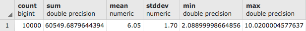
In the summary statistics, if the count indicates less than 10,000 (100²), it means that the raster is 10,000-count/100. In this case, the raster tile is about 0% NODATA.

Let's see how the values of the raster tile are distributed with ST_Histogram():

WITH hist AS ( 
  SELECT (ST_Histogram(rast, 1)).* FROM chp05.prism WHERE rid = 54 
) 
SELECT round(min::numeric, 2) AS min, round(max::numeric, 2) AS max, count, round(percent::numeric, 2) AS percent FROM hist 
ORDER BY min; 

The output will look as follows:

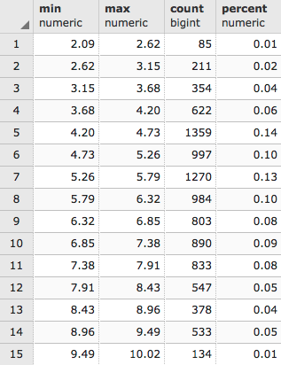
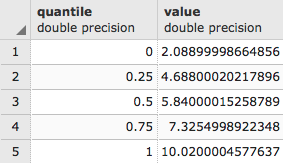
It looks like about 78% of all of the values are at or below 1370.50. Another way to see how the pixel values are distributed is to use ST_Quantile():

SELECT (ST_Quantile(rast, 1)).* 
FROM chp05.prism 
WHERE rid = 54; 

The output of the preceding code is as follows:

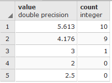
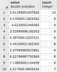
Let's see what the top 10 occurring values are in the raster tile with ST_ValueCount():

SELECT (ST_ValueCount(rast, 1)).* 
FROM chp05.prism WHERE rid = 54 
ORDER BY count DESC, value 
LIMIT 10; 

The output of the code is as follows:

The ST_ValueCount allows other combinations of parameters that will allow rounding up of the values in order to aggregate some of the results, but a previous subset of values to look for must be defined; for example, the following code will count the appearance of values 2, 3, 2.5, 5.612999 and 4.176 rounded to the fifth decimal point 0.00001:

SELECT (ST_ValueCount(rast, 1, true, ARRAY[2,3,2.5,5.612999,4.176]::double precision[] ,0.0001)).* 
FROM chp05.prism 
WHERE rid = 54 
ORDER BY count DESC, value 
LIMIT 10; 

The results show the number of elements that appear similar to the rounded-up values in the array. The two values borrowed from the results on the previous figure, confirm the counting: