Let's generate a slope raster from a subset of our SRTM raster tiles using ST_Slope(). A slope raster computes the rate of elevation change from one pixel to a neighboring pixel:

WITH r AS ( -- union of filtered tiles 
  SELECT ST_Transform(ST_Union(srtm.rast), 3310) AS rast 
  FROM chp05.srtm 
  JOIN chp05.sfpoly sf ON ST_DWithin(ST_Transform(srtm.rast::geometry,  
     3310), ST_Transform(sf.geom, 3310), 1000)),  
  cx AS ( -- custom extent 
    SELECT ST_AsRaster(ST_Transform(sf.geom, 3310), r.rast) AS rast 
    FROM chp05.sfpoly sf CROSS JOIN r 
  ) 
  SELECT ST_Clip(ST_Slope(r.rast, 1, cx.rast), ST_Transform(sf.geom, 3310)) AS rast FROM r 
CROSS JOIN cx 
CROSS JOIN chp05.sfpoly sf; 

All spatial objects in this query are projected to California Albers (SRID 3310), a projection with units in meters. This projection eases the use of ST_DWithin() to broaden our area of interest to include the tiles within 1,000 meters of San Francisco's boundaries, which improves the computed slope values for the pixels at the edges of the San Francisco boundaries. We also use a rasterized version of our San Francisco boundaries as the custom extent for restricting the computed area. After running ST_Slope(), we clip the slope raster just to San Francisco.

We can reuse the ST_Slope() query and substitute ST_HillShade() for ST_Slope() to create a hillshade raster, showing how the sun would illuminate the terrain of the SRTM raster:

WITH r AS ( -- union of filtered tiles 
  SELECT ST_Transform(ST_Union(srtm.rast), 3310) AS rast 
  FROM chp05.srtm 
  JOIN chp05.sfpoly sf ON ST_DWithin(ST_Transform(srtm.rast::geometry,  
    3310), ST_Transform(sf.geom, 3310), 1000)), 
  cx AS ( -- custom extent 
    SELECT ST_AsRaster(ST_Transform(sf.geom, 3310), r.rast) AS rast FROM chp05.sfpoly sf CROSS JOIN r) 
SELECT ST_Clip(ST_HillShade(r.rast, 1, cx.rast),ST_Transform(sf.geom, 3310)) AS rast FROM r 
CROSS JOIN cx 
CROSS JOIN chp05.sfpoly sf; 

In this case, ST_HillShade() is a drop-in replacement for ST_Slope() because we do not specify any special input parameters for either function. If we need to specify additional arguments for ST_Slope() or ST_HillShade(), all changes are confined to just one line.

The following images show the SRTM raster before and after processing it with ST_Slope() and ST_HillShade():

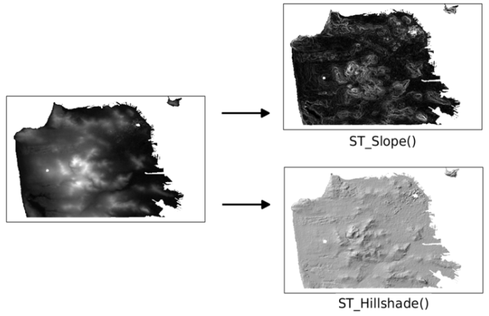
As you can see in the screenshot, the slope and hillshade rasters help us better understand the terrain of San Francisco.

If PostGIS 2.0 is available, we can still use 2.0's ST_Slope() and ST_HillShade() to create slope and hillshade rasters. But there are several differences you need to be aware of, which are as follows:

• ST_Slope() and ST_Aspect() return a raster with values in radians instead of degrees
• Some input parameters of ST_HillShade() are expressed in radians instead of degrees
• The computed raster from ST_Slope(), ST_Aspect(), or ST_HillShade() has an empty 1-pixel border on all four sides

We can adapt our ST_Slope() query from the beginning of this recipe by removing the creation and application of the custom extent. Since the custom extent constrained the computation to just a specific area, the inability to specify such a constraint means PostGIS 2.0's ST_Slope() will perform slower:

WITH r AS ( -- union of filtered tiles 
  SELECT ST_Transform(ST_Union(srtm.rast), 3310) AS rast FROM srtm 
  JOIN sfpoly sf ON ST_DWithin(ST_Transform(srtm.rast::geometry, 3310),
    ST_Transform(sf.geom, 3310), 1000) 
) 
SELECT ST_Clip(ST_Slope(r.rast, 1), ST_Transform(sf.geom, 3310)) AS rast 
FROM r CROSS JOIN sfpoly sf;