Let's adapt part of the query used in the last recipe to find out the average minimum temperature in San Francisco. We replace ST_SummaryStats() with ST_DumpAsPolygons(), and then return the geometries as WKT:

WITH geoms AS (SELECT ST_DumpAsPolygons(ST_Union(ST_Clip(prism.rast, 1, ST_Transform(sf.geom, 4269), TRUE)), 1 ) AS gv 
FROM chp05.prism 
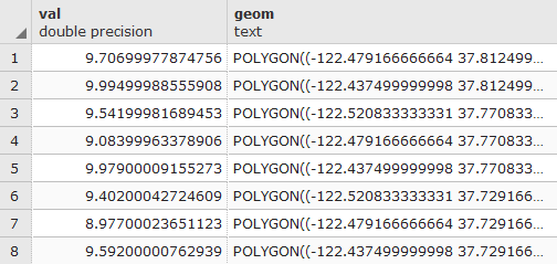
JOIN chp05.sfpoly sf ON ST_Intersects(prism.rast, ST_Transform(sf.geom, 4269)) 
WHERE prism.month_year = '2017-03-01'::date ) 
SELECT (gv).val, ST_AsText((gv).geom) AS geom 
FROM geoms; 

The output is as follows:

Now, replace the ST_DumpAsPolygons() function with ST_PixelsAsPolyons():

WITH geoms AS (SELECT (ST_PixelAsPolygons(ST_Union(ST_Clip(prism.rast, 1, ST_Transform(sf.geom, 4269), TRUE)), 1 )) AS gv 
FROM chp05.prism 
JOIN chp05.sfpoly sf ON ST_Intersects(prism.rast, ST_Transform(sf.geom, 4269)) 
WHERE prism.month_year = '2017-03-01'::date) 
SELECT (gv).val, ST_AsText((gv).geom) AS geom 
FROM geoms; 

The output is as follows:

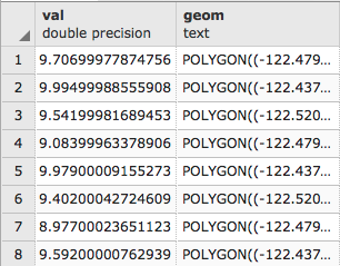
Again, the query results have been trimmed. What is important is the number of rows returned. ST_PixelsAsPolygons() returns significantly more geometries than ST_DumpAsPolygons(). This is due to the different mechanism used in each function.

The following images show the difference between ST_DumpAsPolygons() and ST_PixelsAsPolygons(). The ST_DumpAsPolygons() function only dumps pixels with a value and unites these pixels with the same value. The ST_PixelsAsPolygons() function does not merge pixels and dumps all of them, as shown in the following diagrams:

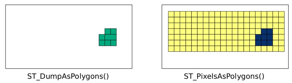
The ST_PixelsAsPolygons() function returns one geometry for each pixel. If there are 100 pixels, there will be 100 geometries. Each geometry of ST_DumpAsPolygons() is the union of all of the pixels in an area with the same value. If there are 100 pixels, there may be up to 100 geometries.

There is one other significant difference between ST_PixelAsPolygons() and ST_DumpAsPolygons(). Unlike ST_DumpAsPolygons(), ST_PixelAsPolygons() returns a geometry for pixels with the NODATA value, and has an empty value for the val column.

Let's convert a geometry to a raster with ST_AsRaster(). We insert ST_AsRaster() to return a raster with a pixel size of 100 by -100 meters containing four bands of the pixel type 8BUI. Each of these bands will have a pixel NODATA value of 0, and a specific pixel value (29, 194, 178, and 255 for each band respectively). The units for the pixel size are determined by the geometry's projection, which is also the projection of the created raster:

SELECT ST_AsRaster( 
  sf.geom, 
  100., -100., 
  ARRAY['8BUI', '8BUI', '8BUI', '8BUI']::text[], 
  ARRAY[29, 194, 178, 255]::double precision[], 
  ARRAY[0, 0, 0, 0]::double precision[] 
) 
FROM sfpoly sf; 

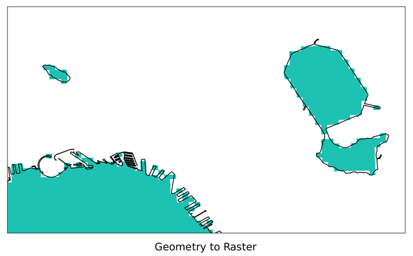
If we visualize the generated raster of San Francisco's boundaries and overlay the source geometry, we get the following result, which is a zoomed-in view of the San Francisco boundary's geometry converted to a raster with ST_AsRaster():

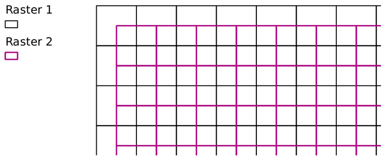
Though it is great that the geometry is now a raster, relating the generated raster to other rasters requires additional processing. This is because the generated raster and the other raster will most likely not be aligned. If the two rasters are not aligned, most PostGIS raster functions do not work. The following figure shows two non-aligned rasters (simplified to pixel grids):

When a geometry needs to be converted to a raster so as to relate to an existing raster, use that existing raster as a reference when calling ST_AsRaster():

SELECT ST_AsRaster( 
  sf.geom, prism.rast, 
  ARRAY['8BUI', '8BUI', '8BUI', '8BUI']::text[], 
  ARRAY[29, 194, 178, 255]::double precision[], 
  ARRAY[0, 0, 0, 0]::double precision[] 
) 
FROM chp05.sfpoly sf 
CROSS JOIN chp05.prism 
WHERE prism.rid = 1; 

In the preceding query, we use the raster tile at rid = 1 as our reference raster. The ST_AsRaster() function uses the reference raster's metadata to create the geometry's raster. If the geometry and reference raster have different SRIDs, the geometry is transformed to the same SRID before creating the raster.