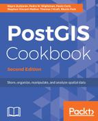
The pgr_drivingdistance polygon we created is the first step in the demographic analysis. Refer to the Driving distance/service area calculation recipe if you need to familiarize yourself with its use. In this case, we'll consider the cycling distance. The nearest node to the Cleveland Metroparks Zoo is 24746, according to our loaded dataset; so we'll use that as the center point for our pgr_drivingdistance calculation and we'll use approximately 6 kilometers as our distance, as we want to know the number of zoo visitors within this distance of the Cleveland Metroparks Zoo. However, since our data is using 4326 EPSG, the distance we will give the function will be in degrees, so 0.05 will give us an approximate distance of 6 km that will work with the pgr_drivingDistance function:

CREATE TABLE chp06.zoo_bikezone AS (
  WITH alphashape AS (
    SELECT pgr_alphaShape('
      WITH DD AS (
        SELECT * FROM pgr_drivingDistance(
          ''SELECT gid AS id, source, target, reverse_cost 
          AS cost FROM chp06.cleveland_ways'',
          24746, 0.05, false
        )
      ),
      dd_points AS(
        SELECT id::int4, ST_X(the_geom)::float8 as x, 
          ST_Y(the_geom)::float8 AS y
        FROM chp06.cleveland_ways_vertices_pgr w, DD d
        WHERE w.id = d.node
      )
      SELECT * FROM dd_points
    ')
  ),
  alphapoints AS (
    SELECT ST_MakePoint((pgr_alphashape).x, (pgr_alphashape).y) 
    FROM alphashape
  ),
  alphaline AS (
    SELECT ST_Makeline(ST_MakePoint) FROM alphapoints
  )
  SELECT 1 as id, ST_SetSRID(ST_MakePolygon(ST_AddPoint(ST_Makeline, ST_StartPoint(ST_Makeline))), 4326) AS the_geom FROM alphaline
);  

The preceding script gives us a very interesting shape (map tiles by Stamen Design, under CC BY 3.0; data by OpenStreetMap, under CC BY SA). See the following screenshot:

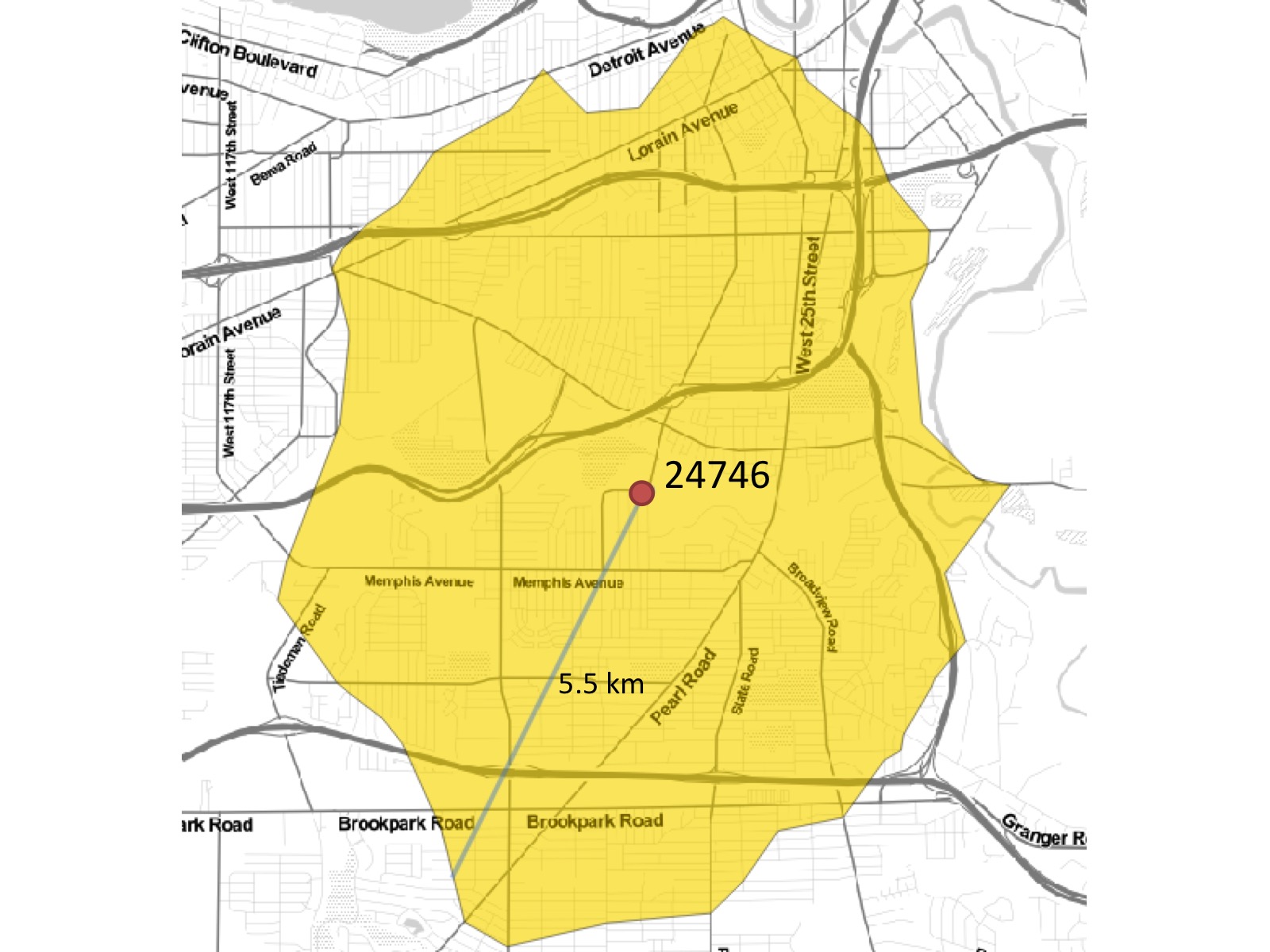
In the previous screenshot, we can see the difference between the cycling distance across the real road network, shaded in blue, and the equivalent 4-mile buffer or as-the-crow-flies distance. Let's apply this to our demographic analysis using the following script:

SELECT ROUND(SUM(chp02.proportional_sum(
  ST_Transform(a.the_geom,3734), b.the_geom, b.pop))) AS population 
FROM Chp06.zoo_bikezone AS a, chp06.census as b
WHERE ST_Intersects(ST_Transform(a.the_geom, 3734), b.the_geom)
GROUP BY a.id;

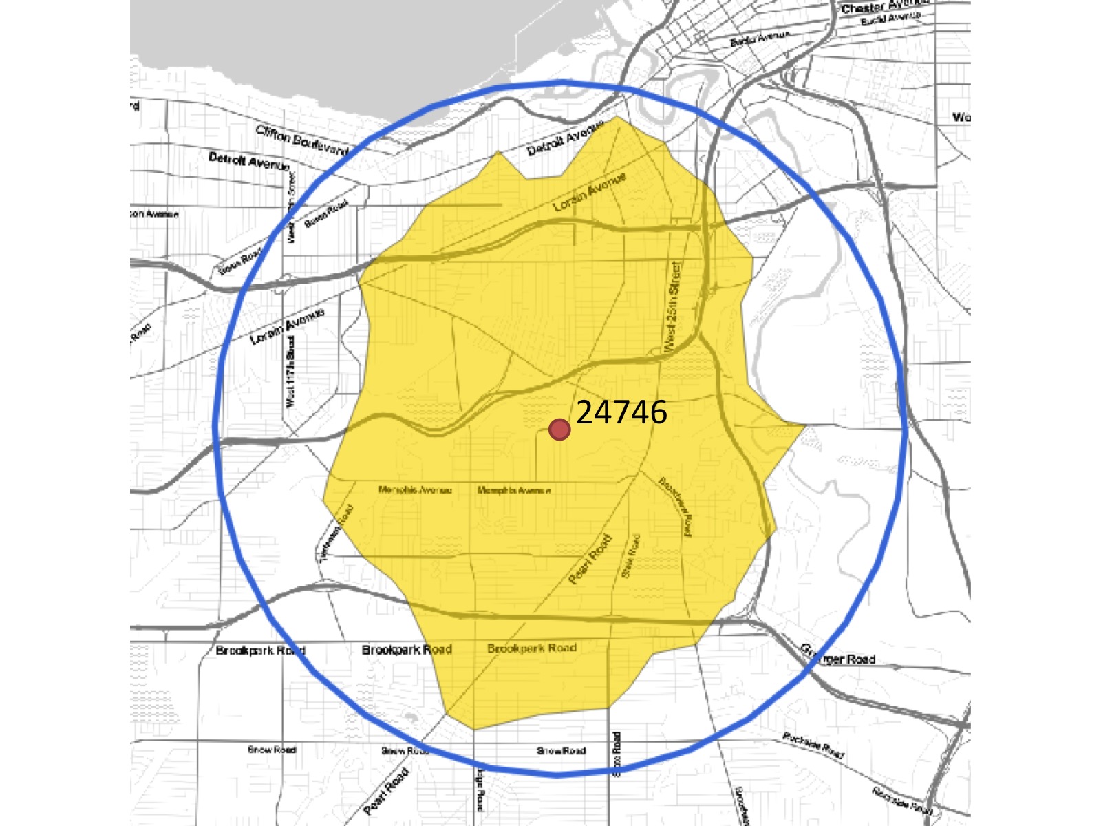
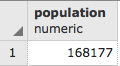
The output is as follows:

(1 row)

So, how does the preceding output compare to what we would get if we look at the buffered distance?

SELECT ROUND(SUM(chp02.proportional_sum(
  ST_Transform(a.the_geom,3734), b.the_geom, b.pop))) AS population 
  FROM (SELECT 1 AS id, ST_Buffer(ST_Transform(the_geom, 3734), 17000) 
    AS the_geom 
  FROM chp06.cleveland_ways_vertices_pgr WHERE id = 24746
) AS a,  chp06.census as b
WHERE ST_Intersects(ST_Transform(a.the_geom, 3734), b.the_geom)
GROUP BY a.id;

(1 row)

The preceding output shows a difference of more than 60,000 people. In other words, using a buffer overestimates the population compared to using pgr_drivingdistance.