Now we are nearly ready for routing. The centerline calculation we have is a good approximation of a straight skeleton, but is still subject to the noisiness of the natural world. We'd like to eliminate that noisiness by choosing our features and emphasizing them through routing. First, we need to prepare the table to allow for routing calculations, as shown in the following commands:

ALTER TABLE chp06.voronoi_intersect ADD COLUMN gid serial;
ALTER TABLE chp06.voronoi_intersect ADD PRIMARY KEY (gid);
    
ALTER TABLE chp06.voronoi_intersect ADD COLUMN source integer;
ALTER TABLE chp06.voronoi_intersect ADD COLUMN target integer;

Then, to create a routable network from our skeleton, enter the following commands:

SELECT pgr_createTopology('voronoi_intersect', 0.001, 'the_geom', 'gid', 'source', 'target', 'true');
    
CREATE INDEX source_idx ON chp06.voronoi_intersect("source");
CREATE INDEX target_idx ON chp06.voronoi_intersect("target");
    
ALTER TABLE chp06.voronoi_intersect ADD COLUMN length double precision;
UPDATE chp06.voronoi_intersect SET length = ST_Length(the_geom);
    
ALTER TABLE chp06.voronoi_intersect ADD COLUMN reverse_cost double precision;
UPDATE chp06.voronoi_intersect SET reverse_cost = length;

Now we can route along the primary centerline of our polygon using the following commands:

CREATE TABLE chp06.voronoi_route AS
WITH dijkstra AS (
  SELECT * FROM pgr_dijkstra('SELECT gid AS id, source, target, length 
    AS cost FROM chp06.voronoi_intersect', 10851, 3, false)
)
    
SELECT gid, geom
FROM voronoi_intersect et, dijkstra d
WHERE et.gid = d.edge;

If we look at the detail of this routing, we see the following:

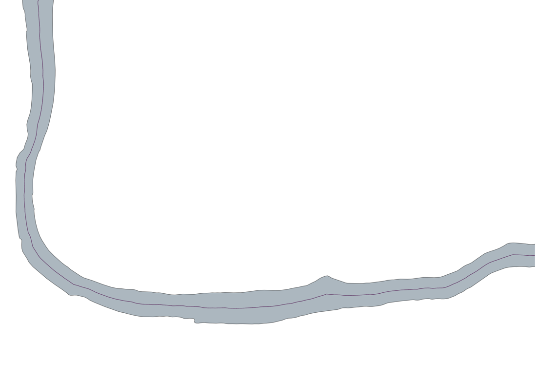
Now we can compare the original polygon with the trace of its centerline:

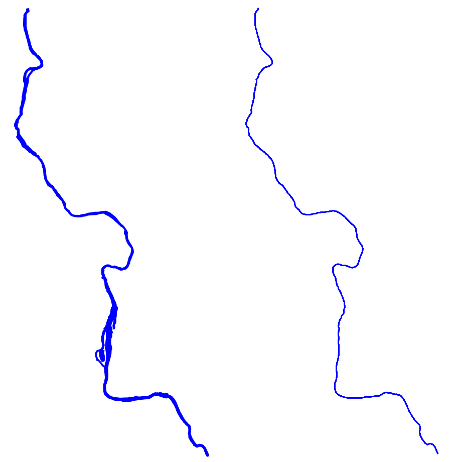
The preceding screenshot shows the original geometry of the stream in contrast to our centerline or skeleton. It is an excellent output that vastly simplifies our input geometry while retaining its relevant features.