Navigate to the DB Manager menu and carry out the following steps:

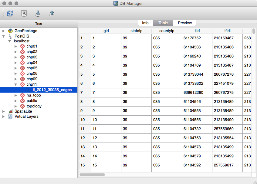
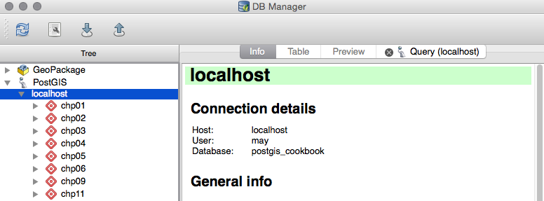
1. Select the tl_2012_39035_edges table in the Tree window.
2. Next, click on the Table tab to view the actual data table, as shown in the following screenshot:

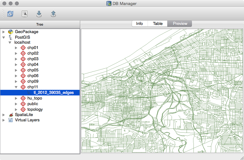
3. The final tab, Preview, is for visualizing the data, as shown in the following screenshot:

To create, modify, and delete database schemas and tables, follow the ensuing steps:

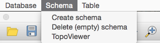
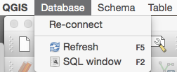
1. First, create a new schema in the database to store data for this chapter. Select Schema | Create schema from the menu bar, as shown in the following screenshot:

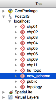
2. Enter new_schema as the schema name and then click on OK. If you do not see the new_schema in the list, you may need to select the database connection in the Tree window and click on the Refresh button or press F5 (see the following screenshot):

Now let's continue to work with our chp11 schema containing the tl_2012_39035_edges table. Let's modify the table name to something more generic. How about lines? You can change the table name by clicking on the table in the Tree window. As soon as the text is highlighted and the cursor flashes, you can delete the existing name and enter the new name, lines.

Right now, our lines table's data is using degrees as the unit of measurement for its current projection (EPSG: 4269). Let's add a new geometry column using EPSG: 3734, which is a State Plane Coordinate system that measures projections in feet. To run SQL queries, follow the ensuing steps:

1. Click on the SQL window button in the DB Manager or press F2, as shown in the following screenshot:

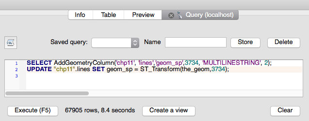
2. Copy the following query into the SQL window and then click on Execute:

      SELECT AddGeometryColumn('chp11', 'lines','geom_sp',3734,
                               'MULTILINESTRING', 2);
      UPDATE "chp11".lines 
      SET geom_sp = ST_Transform(the_geom,3734);

The query creates a new geometry column named geom_sp and then updates the geometry information by transforming the original geometry (geom) from EPSG 4269 to 3734, as shown in the following screenshot:

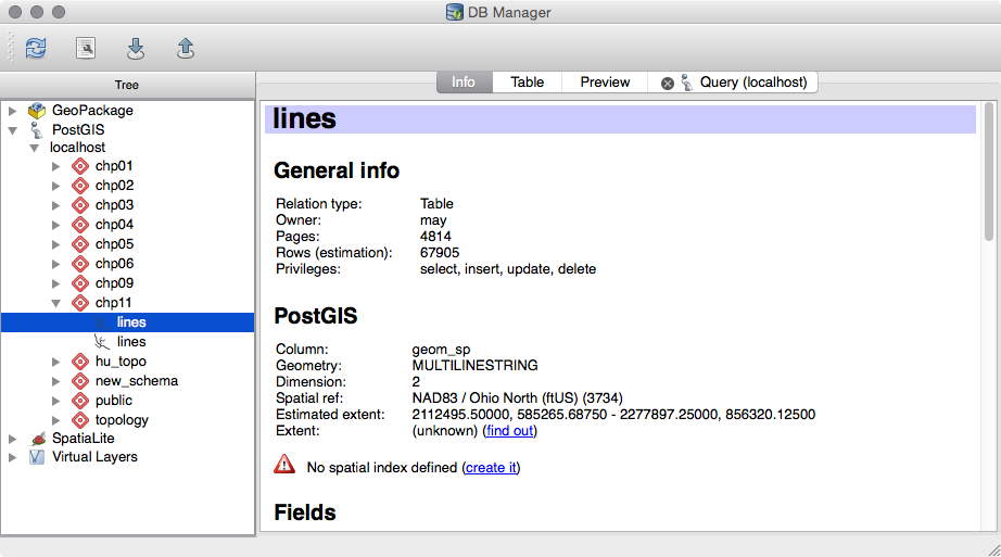
3. Refresh the chp11 schema and you'll notice that the table in the database now has two geometry columns that are treated independently in the Tree window:

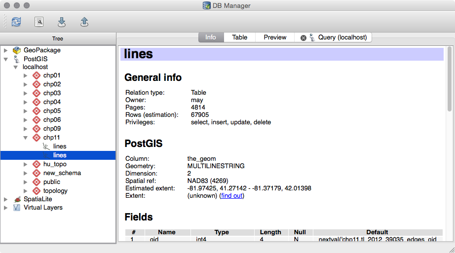
The preceding screenshot shows the original geometry. The following screenshot shows the created geometry:

4. For our next query, let us take a subset of the lines table. Similar to what we did in the preceding section, we will only look at the data about roads. However, this time, we can limit the columns that we want to load with the layer, as well as perform more complicated spatial queries. We'll apply a buffer of 10 feet using the new geometry column (geom_sp) by executing the following command:

      SELECT gid, ST_Buffer(geom_sp, 10) AS geom, fullname, roadflg 
      FROM "chp11".lines WHERE roadflg = 'Y'

Check the Load as new layer checkbox and then select gid as the unique ID and geom as the geometry. Create a name for the layer and then click on Load Now!, and what you'll see is shown in the following screenshot:

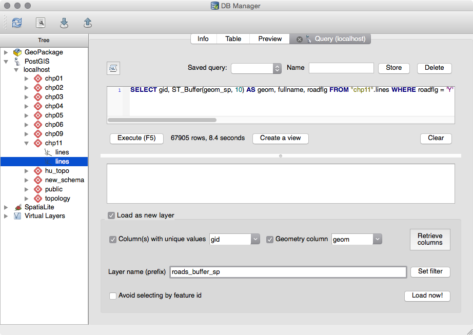
The query adds the result in QGIS as a temporary layer.

5. Now let us modify the query to create a table in the database, rather than load the query as a layer, by executing the following command:

      CREATE TABLE "chp11".roads_buffer_sp AS SELECT gid, 
      ST_Buffer(geom_sp, 10) AS geom, fullname, roadflg 
      FROM "chp11".lines WHERE roadflg = 'Y'

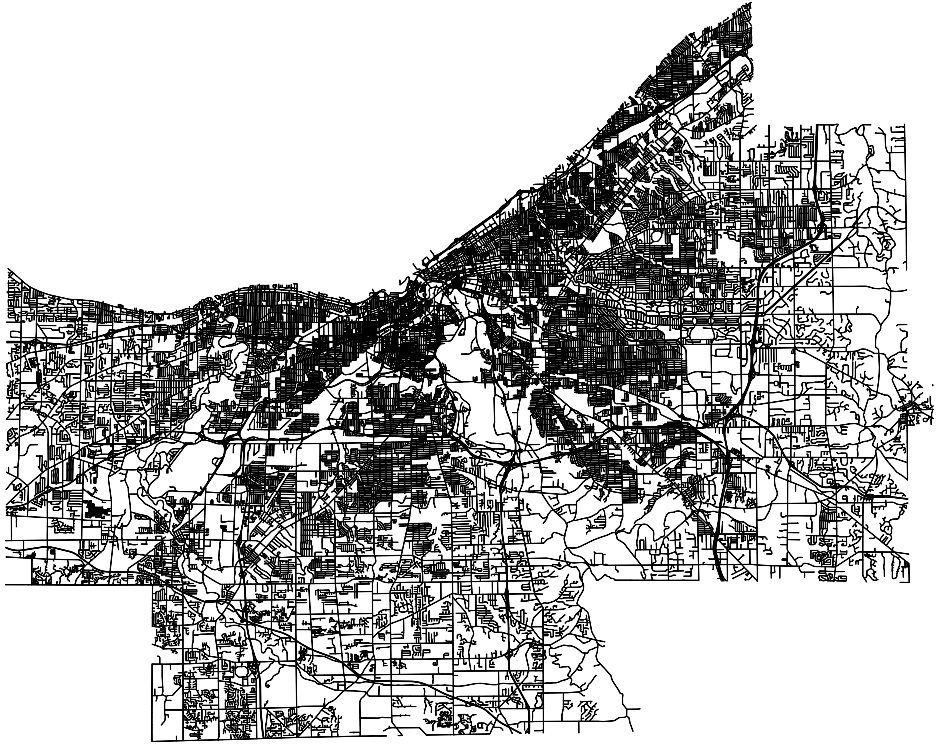
The following screenshot shows the Cuyahoga county road network: