Table of Contents for
PostGIS Cookbook - Second Edition

Version ebook / Retour

Cover image for bash Cookbook, 2nd Edition PostGIS Cookbook - Second Edition by Thomas J Kraft Published by Packt Publishing, 2018
  1. PostGIS Cookbook, Second Edition
  2. Title Page
  3. Copyright and Credits
  4. PostGIS Cookbook Second Edition
  5. Packt Upsell
  6. Why subscribe?
  7. PacktPub.com
  8. Contributors
  9. About the authors
  10. Packt is searching for authors like you
  11. Table of Contents
  12. Preface
  13. Who this book is for
  14. What this book covers
  15. To get the most out of this book
  16. Download the example code files
  17. Download the color images
  18. Conventions used
  19. Sections
  20. Getting ready
  21. How to do it…
  22. How it works…
  23. There's more…
  24. See also
  25. Get in touch
  26. Reviews
  27. Moving Data In and Out of PostGIS
  28. Introduction
  29. Importing nonspatial tabular data (CSV) using PostGIS functions
  30. Getting ready
  31. How to do it...
  32. How it works...
  33. Importing nonspatial tabular data (CSV) using GDAL
  34. Getting ready
  35. How to do it...
  36. How it works...
  37. Importing shapefiles with shp2pgsql
  38. How to do it...
  39. How it works...
  40. There's more...
  41. Importing and exporting data with the ogr2ogr GDAL command
  42. How to do it...
  43. How it works...
  44. See also
  45. Handling batch importing and exporting of datasets
  46. Getting ready
  47. How to do it...
  48. How it works...
  49. Exporting data to a shapefile with the pgsql2shp PostGIS command
  50. How to do it...
  51. How it works...
  52. Importing OpenStreetMap data with the osm2pgsql command
  53. Getting ready
  54. How to do it...
  55. How it works...
  56. Importing raster data with the raster2pgsql PostGIS command
  57. Getting ready
  58. How to do it...
  59. How it works...
  60. Importing multiple rasters at a time
  61. Getting ready
  62. How to do it...
  63. How it works...
  64. Exporting rasters with the gdal_translate and gdalwarp GDAL commands
  65. Getting ready
  66. How to do it...
  67. How it works...
  68. See also
  69. Structures That Work
  70. Introduction
  71. Using geospatial views
  72. Getting ready
  73. How to do it...
  74. How it works...
  75. There's more...
  76. See also
  77. Using triggers to populate the geometry column
  78. Getting ready
  79. How to do it...
  80. There's more...
  81. Extending further...
  82. See also
  83. Structuring spatial data with table inheritance
  84. Getting ready
  85. How to do it...
  86. How it works...
  87. See also
  88. Extending inheritance – table partitioning
  89. Getting ready
  90. How to do it...
  91. How it works...
  92. See also
  93. Normalizing imports
  94. Getting ready
  95. How to do it...
  96. How it works...
  97. There's more...
  98. Normalizing internal overlays
  99. Getting ready
  100. How to do it...
  101. How it works...
  102. There's more...
  103. Using polygon overlays for proportional census estimates
  104. Getting ready
  105. How to do it...
  106. How it works...
  107. Working with Vector Data – The Basics
  108. Introduction
  109. Working with GPS data
  110. Getting ready
  111. How to do it...
  112. How it works...
  113. Fixing invalid geometries
  114. Getting ready
  115. How to do it...
  116. How it works...
  117. GIS analysis with spatial joins
  118. Getting ready
  119. How to do it...
  120. How it works...
  121. Simplifying geometries
  122. How to do it...
  123. How it works...
  124. Measuring distances
  125. Getting ready
  126. How to do it...
  127. How it works...
  128. Merging polygons using a common attribute
  129. Getting ready
  130. How to do it...
  131. How it works...
  132. Computing intersections
  133. Getting ready
  134. How to do it...
  135. How it works...
  136. Clipping geometries to deploy data
  137. Getting ready
  138. How to do it...
  139. How it works...
  140. Simplifying geometries with PostGIS topology
  141. Getting ready
  142. How to do it...
  143. How it works...
  144. Working with Vector Data – Advanced Recipes
  145. Introduction
  146. Improving proximity filtering with KNN
  147. Getting ready
  148. How to do it...
  149. How it works...
  150. See also
  151. Improving proximity filtering with KNN – advanced
  152. Getting ready
  153. How to do it...
  154. How it works...
  155. See also
  156. Rotating geometries
  157. Getting ready
  158. How to do it...
  159. How it works...
  160. See also
  161. Improving ST_Polygonize
  162. Getting ready
  163. How to do it...
  164. See also
  165. Translating, scaling, and rotating geometries – advanced
  166. Getting ready
  167. How to do it...
  168. How it works...
  169. See also
  170. Detailed building footprints from LiDAR
  171. Getting ready
  172. How to do it...
  173. How it works...
  174. Creating a fixed number of clusters from a set of points
  175. Getting ready
  176. How to do it...
  177. Calculating Voronoi diagrams
  178. Getting ready
  179. How to do it...
  180. Working with Raster Data
  181. Introduction
  182. Getting and loading rasters
  183. Getting ready
  184. How to do it...
  185. How it works...
  186. Working with basic raster information and analysis
  187. Getting ready
  188. How to do it...
  189. How it works...
  190. Performing simple map-algebra operations
  191. Getting ready
  192. How to do it...
  193. How it works...
  194. Combining geometries with rasters for analysis
  195. Getting ready
  196. How to do it...
  197. How it works...
  198. Converting between rasters and geometries
  199. Getting ready
  200. How to do it...
  201. How it works...
  202. Processing and loading rasters with GDAL VRT
  203. Getting ready
  204. How to do it...
  205. How it works...
  206. Warping and resampling rasters
  207. Getting ready
  208. How to do it...
  209. How it works...
  210. Performing advanced map-algebra operations
  211. Getting ready
  212. How to do it...
  213. How it works...
  214. Executing DEM operations
  215. Getting ready
  216. How to do it...
  217. How it works...
  218. Sharing and visualizing rasters through SQL
  219. Getting ready
  220. How to do it...
  221. How it works...
  222. Working with pgRouting
  223. Introduction
  224. Startup – Dijkstra routing
  225. Getting ready
  226. How to do it...
  227. Loading data from OpenStreetMap and finding the shortest path using A*
  228. Getting ready
  229. How to do it...
  230. How it works...
  231. Calculating the driving distance/service area
  232. Getting ready
  233. How to do it...
  234. See also
  235. Calculating the driving distance with demographics
  236. Getting ready
  237. How to do it...
  238. Extracting the centerlines of polygons
  239. Getting ready
  240. How to do it...
  241. There's more...
  242. Into the Nth Dimension
  243. Introduction
  244. Importing LiDAR data
  245. Getting ready
  246. How to do it...
  247. See also
  248. Performing 3D queries on a LiDAR point cloud
  249. How to do it...
  250. Constructing and serving buildings 2.5D
  251. Getting ready
  252. How to do it...
  253. Using ST_Extrude to extrude building footprints
  254. How to do it...
  255. Creating arbitrary 3D objects for PostGIS
  256. Getting ready
  257. How to do it...
  258. Exporting models as X3D for the web
  259. Getting ready
  260. How to do it...
  261. There's more...
  262. Reconstructing Unmanned Aerial Vehicle (UAV) image footprints with PostGIS 3D
  263. Getting started
  264. How to do it...
  265. UAV photogrammetry in PostGIS – point cloud
  266. Getting ready
  267. How to do it...
  268. UAV photogrammetry in PostGIS – DSM creation
  269. Getting ready
  270. How to do it...
  271. PostGIS Programming
  272. Introduction
  273. Writing PostGIS vector data with Psycopg
  274. Getting ready
  275. How to do it...
  276. How it works...
  277. Writing PostGIS vector data with OGR Python bindings
  278. Getting ready
  279. How to do it...
  280. How it works...
  281. Writing PostGIS functions with PL/Python
  282. Getting ready
  283. How to do it...
  284. How it works...
  285. Geocoding and reverse geocoding using the GeoNames datasets
  286. Getting ready
  287. How to do it...
  288. How it works...
  289. Geocoding using the OSM datasets with trigrams
  290. Getting ready
  291. How to do it...
  292. How it works...
  293. Geocoding with geopy and PL/Python
  294. Getting ready
  295. How to do it...
  296. How it works...
  297. Importing NetCDF datasets with Python and GDAL
  298. Getting ready
  299. How to do it...
  300. How it works...
  301. PostGIS and the Web
  302. Introduction
  303. Creating WMS and WFS services with MapServer
  304. Getting ready
  305. How to do it...
  306. How it works...
  307. See also
  308. Creating WMS and WFS services with GeoServer
  309. Getting ready
  310. How to do it...
  311. How it works...
  312. See also
  313. Creating a WMS Time service with MapServer
  314. Getting ready
  315. How to do it...
  316. How it works...
  317. Consuming WMS services with OpenLayers
  318. Getting ready
  319. How to do it...
  320. How it works..
  321. Consuming WMS services with Leaflet
  322. How to do it...
  323. How it works...
  324. Consuming WFS-T services with OpenLayers
  325. Getting ready
  326. How to do it...
  327. How it works...
  328. Developing web applications with GeoDjango – part 1
  329. Getting ready
  330. How to do it...
  331. How it works...
  332. Developing web applications with GeoDjango – part 2
  333. Getting ready
  334. How to do it...
  335. How it works...
  336. Developing a web GPX viewer with Mapbox
  337. How to do it...
  338. How it works...
  339. Maintenance, Optimization, and Performance Tuning
  340. Introduction
  341. Organizing the database
  342. Getting ready
  343. How to do it...
  344. How it works...
  345. Setting up the correct data privilege mechanism
  346. Getting ready
  347. How to do it...
  348. How it works...
  349. Backing up the database
  350. Getting ready
  351. How to do it...
  352. How it works...
  353. Using indexes
  354. Getting ready
  355. How to do it...
  356. How it works...
  357. Clustering for efficiency
  358. Getting ready
  359. How to do it...
  360. How it works...
  361. Optimizing SQL queries
  362. Getting ready
  363. How to do it...
  364. How it works...
  365. Migrating a PostGIS database to a different server
  366. Getting ready
  367. How to do it...
  368. How it works...
  369. Replicating a PostGIS database with streaming replication
  370. Getting ready
  371. How to do it...
  372. How it works...
  373. Geospatial sharding
  374. Getting ready
  375. How to do it...
  376. How it works...
  377. Paralellizing in PosgtreSQL
  378. Getting ready
  379. How to do it...
  380. How it works...
  381. Using Desktop Clients
  382. Introduction
  383. Adding PostGIS layers – QGIS
  384. Getting ready
  385. How to do it...
  386. How it works...
  387. Using the Database Manager plugin – QGIS
  388. Getting ready
  389. How to do it...
  390. How it works...
  391. Adding PostGIS layers – OpenJUMP GIS
  392. Getting ready
  393. How to do it...
  394. How it works...
  395. Running database queries – OpenJUMP GIS
  396. Getting ready
  397. How to do it...
  398. How it works...
  399. Adding PostGIS layers – gvSIG
  400. Getting ready
  401. How to do it...
  402. How it works...
  403. Adding PostGIS layers – uDig
  404. How to do it...
  405. How it works...
  406. Introduction to Location Privacy Protection Mechanisms
  407. Introduction
  408. Definition of Location Privacy Protection Mechanisms – LPPMs
  409. Classifying LPPMs
  410. Adding noise to protect location data
  411. Getting ready
  412. How to do it...
  413. How it works...
  414. Creating redundancy in geographical query results
  415. Getting ready
  416. How to do it...
  417. How it works...
  418. References
  419. Other Books You May Enjoy
  420. Leave a review - let other readers know what you think

How to do it...

The following steps will guide you through the iterative process required to improve query performance:

  1. To find a school's nearest police station and the distance between each school in San Francisco and its nearest station, we will start by executing the following query:
      SELECT
        di.school,
        police_address,
        distance
      FROM ( -- for each school, get the minimum distance to a 
-- police station
SELECT gid, school, min(distance) AS distance
FROM ( -- get distance between every school and every police
-- station in San Francisco
SELECT sc.gid, sc.name AS school, po.address AS police_address, ST_Distance(po.geom_3310, sc.geom_3310) AS distance FROM ( -- get schools in San Francisco SELECT ca.gid, ca.name, ST_Transform(ca.geom, 3310) AS geom_3310 FROM sfpoly sf JOIN caschools ca ON ST_Intersects(sf.geom, ST_Transform(ca.geom, 3310)) ) sc CROSS JOIN ( -- get police stations in San Francisco
SELECT
ca.address, ST_Transform(ca.geom, 3310) AS geom_3310
FROM sfpoly sf
JOIN capolice ca ON ST_Intersects(sf.geom, ST_Transform(ca.geom, 3310)) ) po ORDER BY 1, 2, 4 ) scpo GROUP BY 1, 2 ORDER BY 2 ) di JOIN ( -- for each school, collect the police station -- addresses ordered by distance SELECT gid, school, (array_agg(police_address))[1] AS police_address FROM (-- get distance between every school and
every police station in San Francisco
SELECT sc.gid, sc.name AS school, po.address AS police_address, ST_Distance(po.geom_3310, sc.geom_3310) AS distance
FROM ( -- get schools in San Francisco
SELECT ca.gid, ca.name, ST_Transform(ca.geom, 3310) AS geom_3310
FROM sfpoly sf
JOIN caschools ca ON ST_Intersects(sf.geom, ST_Transform(ca.geom, 3310)) ) sc CROSS JOIN ( -- get police stations in San Francisco SELECT ca.address, ST_Transform(ca.geom, 3310) AS geom_3310 FROM sfpoly sf JOIN capolice ca
ON ST_Intersects(sf.geom, ST_Transform(ca.geom, 3310)) ) po ORDER BY 1, 2, 4 ) scpo GROUP BY 1, 2 ORDER BY 2 ) po ON di.gid = po.gid ORDER BY di.school;
  1. Generally speaking, this is a crude and simplistic query. The subquery scpo occurs twice in the query because it needs to compute the shortest distance from a school to its nearest police station and the name of the police station closest to each school. If each instance of scpo took 10 seconds to compute, two instances of scpo would take 20 seconds. This is very detrimental to performance.

Note: the time may vary substantially between experiments, depending on the machine configuration, database usage, and so on. However, the changes in the duration of the experiments will be noticeable and should follow the same improvement ratio presented in this section.

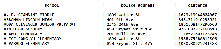
The query output looks as follows:

...
  1. The query results provide the addresses of the schools in San Francisco, the addresses of the closest police station to each of those schools, and the distance from each school to its closest police station. However, we are also interested in getting the answer as fast as possible. With timing turned on in psql, we get the following performance numbers for three runs of the query:
      Time: 5076.363 ms
      Time: 4974.282 ms
      Time: 5027.721 ms
  1. Just by looking at the query in step 1, we can see that there are redundant subqueries. Let's get rid of those duplicates using common table expressions (CTEs), introduced in PostgreSQL 8.4. CTEs are used to logically and syntactically separate a block of SQL from subsequent parts of the query. Since CTEs are logically separated, they are run at the start of the query execution and their results are cached for subsequent use:
      WITH scpo AS ( -- get distance between every school and every 
-- police station in San Francisco
SELECT sc.gid, sc.name AS school, po.address AS police_address, ST_Distance(po.geom_3310, sc.geom_3310) AS distance
FROM ( -- get schools in San Francisco
SELECT ca.*, ST_Transform(ca.geom, 3310) AS geom_3310 FROM sfpoly sf JOIN caschools ca ON ST_Intersects(sf.geom, ST_Transform(ca.geom, 3310)) ) sc CROSS JOIN ( -- get police stations in San Francisco
SELECT
ca.*, ST_Transform(ca.geom, 3310) AS geom_3310 FROM sfpoly sf JOIN capolice ca ON ST_Intersects(sf.geom, ST_Transform(ca.geom, 3310)) ) po ORDER BY 1, 2, 4 ) SELECT di.school, police_address, distance FROM ( -- for each school, get the minimum distance to a -- police station SELECT gid, school, min(distance) AS distance
FROM scpo
GROUP BY 1, 2 ORDER BY 2 ) di JOIN ( -- for each school, collect the police station
-- addresses ordered by distance
SELECT gid, school, (array_agg(police_address))[1] AS police_address FROM scpo GROUP BY 1, 2 ORDER BY 2 ) po ON di.gid = po.gid ORDER BY 1;
  1. Not only is the query syntactically cleaner, but the performance is improved, as shown here:
      Time: 2803.923 ms
      Time: 2798.105 ms
      Time: 2796.481 ms

The execution times went from more than 5 seconds to less than 3 seconds.

  1. Though some may stop optimizing this query at this point, we will continue to improve the query performance. We can use the window functions, which are another PostgreSQL capability introduced in v8.4. Using the window functions as follows, we can get rid of the JOIN expression:
      WITH scpo AS ( -- get distance between every school and every
-- police station in San Francisco
SELECT
sc.name AS school, po.address AS police_address, ST_Distance(po.geom_3310, sc.geom_3310) AS distance
FROM ( -- get schools in San Francisco
SELECT ca.name, ST_Transform(ca.geom, 3310) AS geom_3310 FROM sfpoly sf JOIN caschools ca ON ST_Intersects(sf.geom, ST_Transform(ca.geom, 3310))
) sc
CROSS JOIN ( -- get police stations in San Francisco SELECT ca.address, ST_Transform(ca.geom, 3310) AS geom_3310 FROM sfpoly sf JOIN capolice ca ON ST_Intersects(sf.geom, ST_Transform(ca.geom, 3310)) ) po ORDER BY 1, 3, 2 ) SELECT DISTINCT school, first_value(police_address)
OVER (PARTITION BY school ORDER BY distance),
first_value(distance)
OVER (PARTITION BY school ORDER BY distance)
FROM scpo ORDER BY 1;
  1. We use the first_value() window function to extract the first police_address and distance values for each school sorted by the distance between the school and a police station. The improvement is considerable, reducing from almost 3 seconds to around 1.2 seconds:
      Time: 1261.473 ms
      Time: 1217.843 ms
      Time: 1215.086 ms
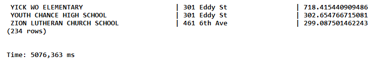
  1. However, it is worth to inspect the execution plan with EXPLAIN ANALYZE VERBOSE to see what is decreasing the query performance. Because of the verbosity of the output, we've trimmed it to just the following lines of interest:
      ...
    
      ->  Nested Loop  (cost=0.15..311.48 rows=1 width=48) 
(actual time=15.047..1186.907 rows=7956 loops=1)
Output: ca.name, ca_1.address,
st_distance(st_transform(ca_1.geom, 3310),
st_transform(ca.geom, 3310))
  1. In the EXPLAIN ANALYZE VERBOSE output, we want to inspect the values for the actual time, which provide the actual start and end times for that part of the query. Of all the actual time ranges, the actual time value of 15.047..1186.907 for the Nested Loop (highlighted in the preceding output) is the worst. This query step consumes at least 80 percent of the total execution time, so any work done to improve performance must be done in this step.
  1. The columns returned from the slow Nested Loop utility are found in the value for the output. Of these columns, st_distance() is present only in this step and not in any inner step. This means we will need to mitigate the number of calls to ST_Distance().
  2. At this step, further query improvements are not possible without running PostgreSQL 9.1 or a later version. PostgreSQL 9.1 introduced indexed nearest-neighbor searches using the <-> and <#> operators to compare the geometries' convex hulls and bounding boxes, respectively. For point geometries, both operators result in the same answer.
  3. Let's rewrite the query to take advantage of the <-> operator. The following query still uses the CTEs and window functions:
      WITH sc AS ( -- get schools in San Francisco
        SELECT
          ca.gid,
          ca.name,
          ca.geom
        FROM sfpoly sf
        JOIN caschools ca
          ON ST_Intersects(sf.geom, ST_Transform(ca.geom, 3310))
      ), po AS ( -- get police stations in San Francisco
        SELECT
          ca.gid,
          ca.address,
          ca.geom
        FROM sfpoly sf
        JOIN capolice ca
          ON ST_Intersects(sf.geom, ST_Transform(ca.geom, 3310))
      )
      SELECT
        school,
        police_address,
        ST_Distance(ST_Transform(school_geom, 3310), 
ST_Transform(police_geom, 3310)) AS distance
FROM ( -- for each school, number and order the police
-- stations by how close each station is to the school
SELECT ROW_NUMBER() OVER (
PARTITION BY sc.gid ORDER BY sc.geom <-> po.geom
) AS r,
sc.name AS school, sc.geom AS school_geom, po.address AS police_address, po.geom AS police_geom FROM sc CROSS JOIN po ) scpo WHERE r < 2 ORDER BY 1;
  1. The query has the following performance numbers:
      Time: 83.002 ms
      Time: 82.586 ms
      Time: 83.327 ms

Wow! Using indexed nearest-neighbor searches with the <-> operator, we reduced our initial query from one second to less than a tenth of a second.