Download VisualSFM from http://ccwu.me/vsfm/. In a console terminal, execute the following:

Visualsfm <IMAGES_FOLDER>

VisualSFM will start rendering the 3D, model using as input a folder with images. It will take a couple of hours to process. Then, when it finishes, it will return a point cloud file.

We can view this data in a program such as MeshLab at http://meshlab.sourceforge.net/. A good tutorial on using MeshLab to view point clouds can be found at http://www.cse.iitd.ac.in/~mcs112609/Meshlab%20Tutorial.pdf.

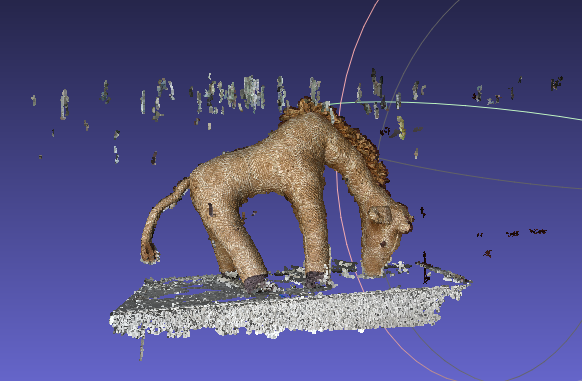
The following image shows what our point cloud looks like when viewed in MeshLab:

In the VisualSFM output, there is a file with the extension .ply, for example, giraffe.ply (included in the source code for this chapter). If you open this file in a text editor, it will look something like the following:

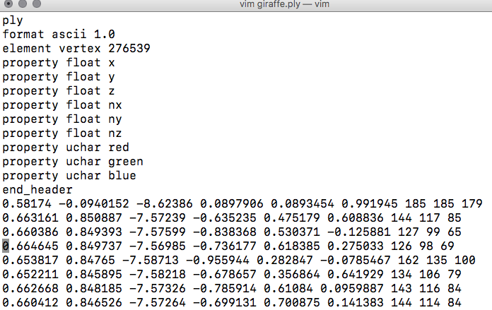
This is the header portion of our file. It specifies the .ply format, the encoding format ascii 1.0, the number of vertices, and then the column names for all the data returned: x, y, z, nx, ny, nz, red, green, and blue.

For importing into PostGIS, we will import all the fields, but will focus on x, y, and z for our point cloud, as well as look at color. For our purposes, this file specifies relative x, y, and z coordinates, and the color of each of those points in channels red, green, and blue. These colors are 24-bit colors—and thus they can have integer values between 0 and 255.

For the remainder of the recipe, we will create a PDAL pipeline, modifying the JSON structure reader to be a .ply file. Check the recipe for Importing LiDAR data in this chapter to see how to create a PDAL pipeline:

{
  "pipeline": [{
    "type": "readers.ply",
    "filename": "/data/giraffe/giraffe.ply"
  }, {
    "type": "writers.pgpointcloud",
    "connection": "host='localhost' dbname='postgis-cookbook' user='me' 
     password='me' port='5432'",
    "table": "giraffe",
    "srid": "3734",
    "schema": "chp07"
  }]
}  

Then we execute in the Terminal:

$ pdal pipeline giraffe.json"

This output will serve us for input in the next recipe.