PostGIS Cookbook
Second Edition
Second Edition
Store, organize, manipulate, and analyze spatial data

BIRMINGHAM - MUMBAI
Copyright © 2018 Packt Publishing
All rights reserved. No part of this book may be reproduced, stored in a retrieval system, or transmitted in any form or by any means, without the prior written permission of the publisher, except in the case of brief quotations embedded in critical articles or reviews.
Every effort has been made in the preparation of this book to ensure the accuracy of the information presented. However, the information contained in this book is sold without warranty, either express or implied. Neither the authors, nor Packt Publishing or its dealers and distributors, will be held liable for any damages caused or alleged to have been caused directly or indirectly by this book.
Packt Publishing has endeavored to provide trademark information about all of the companies and products mentioned in this book by the appropriate use of capitals. However, Packt Publishing cannot guarantee the accuracy of this information.
Commissioning Editor: Merint Mathew
Acquisition Editors: Nitin Dasan, Shriram Shekhar
Content Development Editor: Nikhil Borkar
Technical Editor: Subhalaxmi Nadar
Copy Editor: Safis Editing
Project Coordinator: Ulhas Kambali
Proofreader: Safis Editing
Indexer: Mariammal Chettiyar
Graphics: Tania Dutta
Production Coordinator: Shantanu Zagade
First published: January 2014
Second edition: March 2018
Production reference: 1270318
Published by Packt Publishing Ltd.
Livery Place
35 Livery Street
Birmingham
B3 2PB, UK.
ISBN 978-1-78829-932-9

Mapt is an online digital library that gives you full access to over 5,000 books and videos, as well as industry leading tools to help you plan your personal development and advance your career. For more information, please visit our website.
Spend less time learning and more time coding with practical eBooks and Videos from over 4,000 industry professionals
Improve your learning with Skill Plans built especially for you
Get a free eBook or video every month
Mapt is fully searchable
Copy and paste, print, and bookmark content
Did you know that Packt offers eBook versions of every book published, with PDF and ePub files available? You can upgrade to the eBook version at www.PacktPub.com and as a print book customer, you are entitled to a discount on the eBook copy. Get in touch with us at service@packtpub.com for more details.
At www.PacktPub.com, you can also read a collection of free technical articles, sign up for a range of free newsletters, and receive exclusive discounts and offers on Packt books and eBooks.
Mayra Zurbarán is a Colombian geogeek currently pursuing her PhD in geoprivacy. She has a BS in computer science from Universidad del Norte and is interested in the intersection of ethical location data management, free and open source software, and GIS. She is a Pythonista with a marked preference for the PostgreSQL database. Mayra is a member of the Geomatics and Earth Observation laboratory (GEOlab) at Politecnico di Milano and is also a contributor to the FOSS community.
Pedro M. Wightman is an associate professor at the Systems Engineering Department of Universidad del Norte, Barranquilla, Colombia. With a PhD in computer science from the University of South Florida, he's a researcher in location-based information systems, wireless sensor networks, and virtual and augmented reality, among other fields. Father of two beautiful and smart girls, he's also a rookie writer of short stories, science fiction fan, time travel enthusiast, and is worried about how to survive apocalyptic solar flares.
Paolo Corti is an environmental engineer with 20 years of experience in the GIS field, currently working as a Geospatial Engineer Fellow at the Center for Geographic Analysis at Harvard University. He is an advocate of open source geospatial technologies and Python, an OSGeo Charter member, and a member of the pycsw and GeoNode Project Steering Committees. He is a coauthor of the first edition of this book and the reviewer for the first and second editions of the Mastering QGIS book by Packt.
Stephen Vincent Mather has worked in the geospatial industry for 15 years, having always had a flair for geospatial analyses in general, especially those at the intersection of Geography and Ecology. His work in open-source geospatial databases started 5 years ago with PostGIS and he immediately began using PostGIS as an analytic tool, attempting a range of innovative and sometimes bleeding-edge techniques (although he admittedly prefers the cutting edge).
Thomas J Kraft is currently a Planning Technician at Cleveland Metroparks after beginning as a GIS intern in 2011. He graduated with Honors from Cleveland State University in 2012, majoring in Environmental Science with an emphasis on GIS. When not in front of a computer, he spends his weekends landscaping and in the outdoors in general.
Bborie Park has been breaking (and subsequently fixing) computers for most of his life. His primary interests involve developing end-to-end pipelines for spatial datasets. He is an active contributor to the PostGIS project and is a member of the PostGIS Steering Committee. He happily resides with his wife Nicole in the San Francisco Bay Area.
If you're interested in becoming an author for Packt, please visit authors.packtpub.com and apply today. We have worked with thousands of developers and tech professionals, just like you, to help them share their insight with the global tech community. You can make a general application, apply for a specific hot topic that we are recruiting an author for, or submit your own idea.
How close is the nearest hospital from my children's school? Where were the property crimes in my city for the last three months? What is the shortest route from my home to my office? What route should I prescribe for my company's delivery truck to maximize equipment utilization and minimize fuel consumption? Where should the next fire station be built to minimize response times?
People ask these questions, and others like them, every day all over this planet. Answering these questions requires a mechanism capable of thinking in two or more dimensions. Historically, desktop GIS applications were the only ones capable of answering these questions. This method—though completely functional—is not viable for the average person; most people do not need all the functionalities that these applications can offer, or they do not know how to use them. In addition, more and more location-based services offer the specific features that people use and are accessible even from their smartphones. Clearly, the massification of these services requires the support of a robust backend platform to process a large number of geographical operations.
Since scalability, support for large datasets, and a direct input mechanism are required or desired, most developers have opted to adopt spatial databases as their support platform. There are several spatial database software available, some proprietary and others open source. PostGIS is an open source spatial database software available, and probably the most accessible of all spatial database software.
PostGIS runs as an extension to provide spatial capabilities to PostgreSQL databases. In this capacity, PostGIS permits the inclusion of spatial data alongside data typically found in a database. By having all the data together, questions such as "What is the rank of all the police stations, after taking into account the distance for each response time?" are possible. New or enhanced capabilities are possible by building upon the core functions provided by PostGIS and the inherent extensibility of PostgreSQL. Furthermore, this book also includes an invitation to include location privacy protection mechanisms in new GIS applications and in location-based services so that users feel respected and not necessarily at risk for sharing their information, especially information as sensitive as their whereabouts.
PostGIS Cookbook, Second Edition uses a problem-solving approach to help you acquire a solid understanding of PostGIS. It is hoped that this book provides answers to some common spatial questions and gives you the inspiration and confidence to use and enhance PostGIS in finding solutions to challenging spatial problems.
This book is written for those who are looking for the best method to solve their spatial problems using PostGIS. These problems can be as simple as finding the nearest restaurant to a specific location, or as complex as finding the shortest and/or most efficient route from point A to point B.
For readers who are just starting out with PostGIS, or even with spatial datasets, this book is structured to help them become comfortable and proficient at running spatial operations in the database. For experienced users, the book provides opportunities to dive into advanced topics such as point clouds, raster map-algebra, and PostGIS programming.
Chapter 1, Moving Data In and Out of PostGIS, covers the processes available for importing and exporting spatial and non-spatial data to and from PostGIS. These processes include the use of utilities provided by PostGIS and by third parties, such as GDAL/OGR.
Chapter 2, Structures That Work, discusses how to organize PostGIS data using mechanisms available through PostgreSQL. These mechanisms are used to normalize potentially unclean and unstructured import data.
Chapter 3, Working with Vector Data – The Basics, introduces PostGIS operations commonly done on vectors, known as geometries and geographies in PostGIS. Operations covered include the processing of invalid geometries, determining relationships between geometries, and simplifying complex geometries.
Chapter 4, Working with Vector Data – Advanced Recipes, dives into advanced topics for analyzing geometries. You will learn how to make use of KNN filters to increase the performance of proximity queries, create polygons from LiDAR data, and compute Voronoi cells usable in neighborhood analyses.
Chapter 5, Working with Raster Data, presents a realistic workflow for operating on rasters in PostGIS. You will learn how to import a raster, modify the raster, conduct analysis on the raster, and export the raster in standard raster formats.
Chapter 6, Working with pgRouting, introduces the pgRouting extension, which brings graph traversal and analysis capabilities to PostGIS. The recipes in this chapter answer real-world questions of conditionally navigating from point A to point B and accurately modeling complex routes, such as waterways.
Chapter 7, Into the Nth Dimension, focuses on the tools and techniques used to process and analyze multidimensional spatial data in PostGIS, including LiDAR-sourced point clouds. Topics covered include the loading of point clouds into PostGIS, creating 2.5D and 3D geometries from point clouds, and the application of several photogrammetry principles.
Chapter 8, PostGIS Programming, shows how to use the Python language to write applications that operate on and interact with PostGIS. The applications written include methods to read and write external datasets to and from PostGIS, as well as a basic geocoding engine using OpenStreetMap datasets.
Chapter 9, PostGIS and the Web, presents the use of OGC and REST web services to deliver PostGIS data and services to the web. This chapter discusses providing OGC, WFS, and WMS services with MapServer and GeoServer, and consuming them from clients such as OpenLayers and Leaflet. It then shows how to build a web application with GeoDjango and how to include your PostGIS data in a Mapbox application.
Chapter 10, Maintenance, Optimization, and Performance Tuning, takes a step back from PostGIS and focuses on the capabilities of the PostgreSQL database server. By leveraging the tools provided by PostgreSQL, you can ensure the long-term viability of your spatial and non-spatial data, and maximize the performance of various PostGIS operations. In addition, it explores new features such as geospatial sharding and parallelism in PostgreSQL.
Chapter 11, Using Desktop Clients, tells you about how spatial data in PostGIS can be consumed and manipulated using various open source desktop GIS applications. Several applications are discussed so as to highlight the different approaches to interacting with spatial data and help you find the right tool for the task.
Chapter 12, Introduction to Location Privacy Protection Mechanisms, provides an introductory approximation to the concept of location privacy and presents the implementation of two different location privacy protection mechanisms that can be included in commercial applications to give a basic level of protection to the user's location data.
Before going further into this book, you will want to install latest versions of PostgreSQL and PostGIS (9.6 or 103 and 2.3 or 2.41, respectively). You may also want to install pgAdmin (1.18) if you prefer a graphical SQL tool. For most computing environments (Windows, Linux, macOS X), installers and packages include all required dependencies of PostGIS. The minimum required dependencies for PostGIS are PROJ.4, GEOS, libjson and GDAL.
A basic understanding of the SQL language is required to understand and adapt the code found in this book's recipes.
You can download the example code files for this book from your account at www.packtpub.com. If you purchased this book elsewhere, you can visit www.packtpub.com/support and register to have the files emailed directly to you.
You can download the code files by following these steps:
Once the file is downloaded, please make sure that you unzip or extract the folder using the latest version of:
The code bundle for the book is also hosted on GitHub at https://github.com/PacktPublishing/PostGIS-Cookbook-Second-Edition. In case there's an update to the code, it will be updated on the existing GitHub repository.
We also have other code bundles from our rich catalog of books and videos available at https://github.com/PacktPublishing/. Check them out!
We also provide a PDF file that has color images of the screenshots/diagrams used in this book. You can download it here: https://www.packtpub.com/sites/default/files/downloads/PostGISCookbookSecondEdition_ColorImages.pdf.
There are a number of text conventions used throughout this book.
CodeInText: Indicates code words in text, database table names, folder names, filenames, file extensions, pathnames, dummy URLs, user input, and Twitter handles. Here is an example: "We will import the firenews.csv file that stores a series of web news collected from various RSS feeds."
A block of code is set as follows:
SELECT ROUND(SUM(chp02.proportional_sum(ST_Transform(a.geom,3734), b.geom, b.pop))) AS population
  FROM nc_walkzone AS a, census_viewpolygon as b
  WHERE ST_Intersects(ST_Transform(a.geom, 3734), b.geom)
  GROUP BY a.id;
When we wish to draw your attention to a particular part of a code block, the relevant lines or items are set in bold:
SELECT ROUND(SUM(chp02.proportional_sum(ST_Transform(a.geom,3734), b.geom, b.pop))) AS population
  FROM nc_walkzone AS a, census_viewpolygon as b
  WHERE ST_Intersects(ST_Transform(a.geom, 3734), b.geom)
  GROUP BY a.id;
Any command-line input or output is written as follows:
> raster2pgsql -s 4322 -t 100x100 -F -I -C -Y C:\postgis_cookbook\data\chap5\PRISM\us_tmin_2012.*.asc chap5.prism | psql -d postgis_cookbook
Bold: Indicates a new term, an important word, or words that you see onscreen. For example, words in menus or dialog boxes appear in the text like this. Here is an example: "Clicking the Next button moves you to the next screen."
In this book, you will find several headings that appear frequently (Getting ready, How to do it..., How it works..., There's more..., and See also).
To give clear instructions on how to complete a recipe, use these sections as follows:
This section tells you what to expect in the recipe and describes how to set up any software or any preliminary settings required for the recipe.
This section contains the steps required to follow the recipe.
This section usually consists of a detailed explanation of what happened in the previous section.
This section consists of additional information about the recipe in order to make you more knowledgeable about the recipe.
This section provides helpful links to other useful information for the recipe.
Feedback from our readers is always welcome.
General feedback: Email feedback@packtpub.com and mention the book title in the subject of your message. If you have questions about any aspect of this book, please email us at questions@packtpub.com.
Errata: Although we have taken every care to ensure the accuracy of our content, mistakes do happen. If you have found a mistake in this book, we would be grateful if you would report this to us. Please visit www.packtpub.com/submit-errata, selecting your book, clicking on the Errata Submission Form link, and entering the details.
Piracy: If you come across any illegal copies of our works in any form on the internet, we would be grateful if you would provide us with the location address or website name. Please contact us at copyright@packtpub.com with a link to the material.
If you are interested in becoming an author: If there is a topic that you have expertise in and you are interested in either writing or contributing to a book, please visit authors.packtpub.com.
Please leave a review. Once you have read and used this book, why not leave a review on the site that you purchased it from? Potential readers can then see and use your unbiased opinion to make purchase decisions, we at Packt can understand what you think about our products, and our authors can see your feedback on their book. Thank you!
For more information about Packt, please visit packtpub.com.
In this chapter, we will cover:
PostGIS is an open source extension for the PostgreSQL database that allows support for geographic objects; throughout this book you will find recipes that will guide you step by step to explore the different functionalities it offers.
The purpose of the book is to become a useful tool for understanding the capabilities of PostGIS and how to apply them in no time. Each recipe presents a preparation stage, in order to organize your workspace with everything you may need, then the set of steps that you need to perform in order to achieve the main goal of the task, that includes all the external commands and SQL sentences you will need (which have been tested in Linux, Mac and Windows environments), and finally a small summary of the recipe. This book will go over a large set of common tasks in geographical information systems and location-based services, which makes it a must-have book in your technical library.
In this first chapter, we will show you a set of recipes covering different tools and methodologies to import and export geographic data from the PostGIS spatial database, given that pretty much every common action to perform in a GIS starts with inserting or exporting geospatial data.
There are a couple of alternative approaches to importing a Comma Separated Values (CSV) file, which stores attributes and geometries in PostGIS. In this recipe, we will use the approach of importing such a file using the PostgreSQL COPY command and a couple of PostGIS functions.
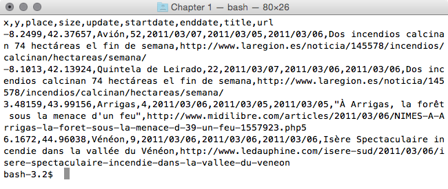
We will import the firenews.csv file that stores a series of web news collected from various RSS feeds related to forest fires in Europe in the context of the European Forest Fire Information System (EFFIS), available at http://effis.jrc.ec.europa.eu/.
For each news feed, there are attributes such as place name, size of the fire in hectares, URL, and so on. Most importantly, there are the x and y fields that give the position of the geolocalized news in decimal degrees (in the WGS 84 spatial reference system, SRID = 4326).
For Windows machines, it is necessary to install OSGeo4W, a set of open source geographical libraries that will allow the manipulation of the datasets. The link is: https://trac.osgeo.org/osgeo4w/
In addition, include the OSGeo4W and the Postgres binary folders in the Path environment variable to be able to execute the commands from any location in your PC.
The steps you need to follow to complete this recipe are as shown:
      $ cd ~/postgis_cookbook/data/chp01/
      $ head -n 5 firenews.csv
The output of the preceding command is as shown:
      $ psql -U me -d postgis_cookbook
      postgis_cookbook=> CREATE EXTENSION postgis;
      postgis_cookbook=> CREATE SCHEMA chp01;
      postgis_cookbook=> CREATE TABLE chp01.firenews
      (
        x float8,
        y float8,
        place varchar(100),
        size float8,
        update date,
        startdate date,
        enddate date,
        title varchar(255),
        url varchar(255),
        the_geom geometry(POINT, 4326)
      );
      postgis_cookbook=> COPY chp01.firenews (
        x, y, place, size, update, startdate,
        enddate, title, url
      ) FROM '/tmp/firenews.csv' WITH CSV HEADER;
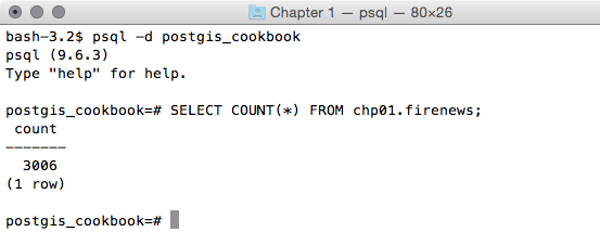
postgis_cookbook=> SELECT COUNT(*) FROM chp01.firenews;
The output of the preceding command is as follows:
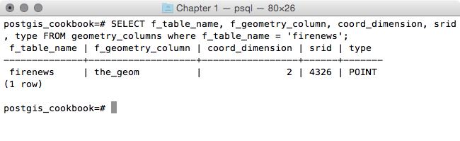
     postgis_cookbook=# SELECT f_table_name,
     f_geometry_column, coord_dimension, srid, type
     FROM geometry_columns where f_table_name = 'firenews';
The output of the preceding command is as follows:
In PostGIS 2.0, you can still use the AddGeometryColumn function if you wish; however, you need to set its use_typmod parameter to false.
      postgis_cookbook=> UPDATE chp01.firenews
      SET the_geom = ST_SetSRID(ST_MakePoint(x,y), 4326);
      postgis_cookbook=> UPDATE chp01.firenews
      SET the_geom = ST_PointFromText('POINT(' || x || ' ' || y || ')',
                                      4326);
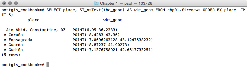
      postgis_cookbook=# SELECT place, ST_AsText(the_geom) AS wkt_geom
      FROM chp01.firenews ORDER BY place LIMIT 5;
The output of the preceding comment is as follows:
      postgis_cookbook=> CREATE INDEX idx_firenews_geom
      ON chp01.firenews USING GIST (the_geom);
This recipe showed you how to load nonspatial tabular data (in CSV format) in PostGIS using the COPY PostgreSQL command.
After creating the table and copying the CSV file rows to the PostgreSQL table, you updated the geometric column using one of the geometry constructor functions that PostGIS provides (ST_MakePoint and ST_PointFromText for bi-dimensional points).
These geometry constructors (in this case, ST_MakePoint and ST_PointFromText) must always provide the spatial reference system identifier (SRID) together with the point coordinates to define the point geometry.
Each geometric field added in any table in the database is tracked with a record in the geometry_columns PostGIS metadata view. In the previous PostGIS version (< 2.0), the geometry_fields view was a table and needed to be manually updated, possibly with the convenient AddGeometryColumn function.
For the same reason, to maintain the updated geometry_columns view when dropping a geometry column or removing a spatial table in the previous PostGIS versions, there were the DropGeometryColumn and DropGeometryTable functions. With PostGIS 2.0 and newer, you don't need to use these functions any more, but you can safely remove the column or the table with the standard ALTER TABLE, DROP COLUMN, and DROP TABLE SQL commands.
In the last step of the recipe, you have created a spatial index on the table to improve performance. Please be aware that as in the case of alphanumerical database fields, indexes improve performances only when reading data using the SELECT command. In this case, you are making a number of updates on the table (INSERT, UPDATE, and DELETE); depending on the scenario, it could be less time consuming to drop and recreate the index after the updates.
As an alternative approach to the previous recipe, you will import a CSV file to PostGIS using the ogr2ogr GDAL command and the GDAL OGR virtual format. The Geospatial Data Abstraction Library (GDAL) is a translator library for raster geospatial data formats. OGR is the related library that provides similar capabilities for vector data formats.
This time, as an extra step, you will import only a part of the features in the file and you will reproject them to a different spatial reference system.
You will import the Global_24h.csv file to the PostGIS database from NASA's Earth Observing System Data and Information System (EOSDIS).
You can copy the file from the dataset directory of the book for this chapter.
This file represents the active hotspots in the world detected by the Moderate Resolution Imaging Spectroradiometer (MODIS) satellites in the last 24 hours. For each row, there are the coordinates of the hotspot (latitude, longitude) in decimal degrees (in the WGS 84 spatial reference system, SRID = 4326), and a series of useful fields such as the acquisition date, acquisition time, and satellite type, just to name a few.
You will import only the active fire data scanned by the satellite type marked as T (Terra MODIS), and you will project it using the Spherical Mercator projection coordinate system (EPSG:3857; it is sometimes marked as EPSG:900913, where the number 900913 represents Google in 1337 speak, as it was first widely used by Google Maps).
The steps you need to follow to complete this recipe are as follows:
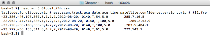
      $ cd ~/postgis_cookbook/data/chp01/
      $ head -n 5 Global_24h.csv
The output of the preceding command is as follows:
       <OGRVRTDataSource>
         <OGRVRTLayer name="Global_24h">
         <SrcDataSource>Global_24h.csv</SrcDataSource>
         <GeometryType>wkbPoint</GeometryType>
         <LayerSRS>EPSG:4326</LayerSRS>
           <GeometryField encoding="PointFromColumns"
            x="longitude" y="latitude"/>
         </OGRVRTLayer>
       </OGRVRTDataSource>
$ ogrinfo global_24h.vrt Global_24h -fid 1
The output of the preceding command is as follows:

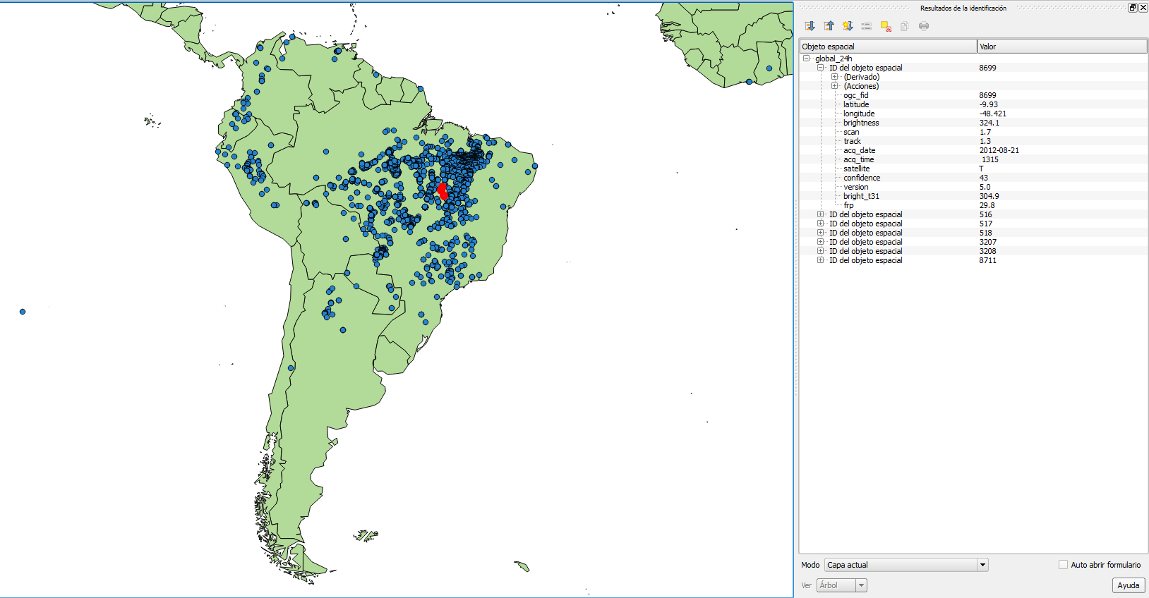
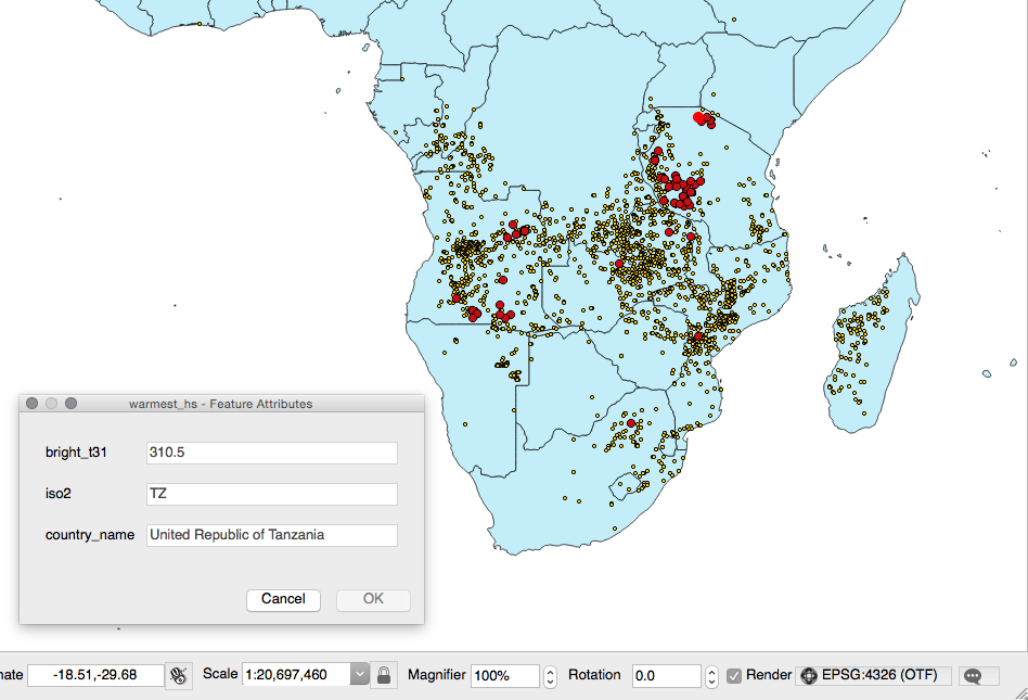
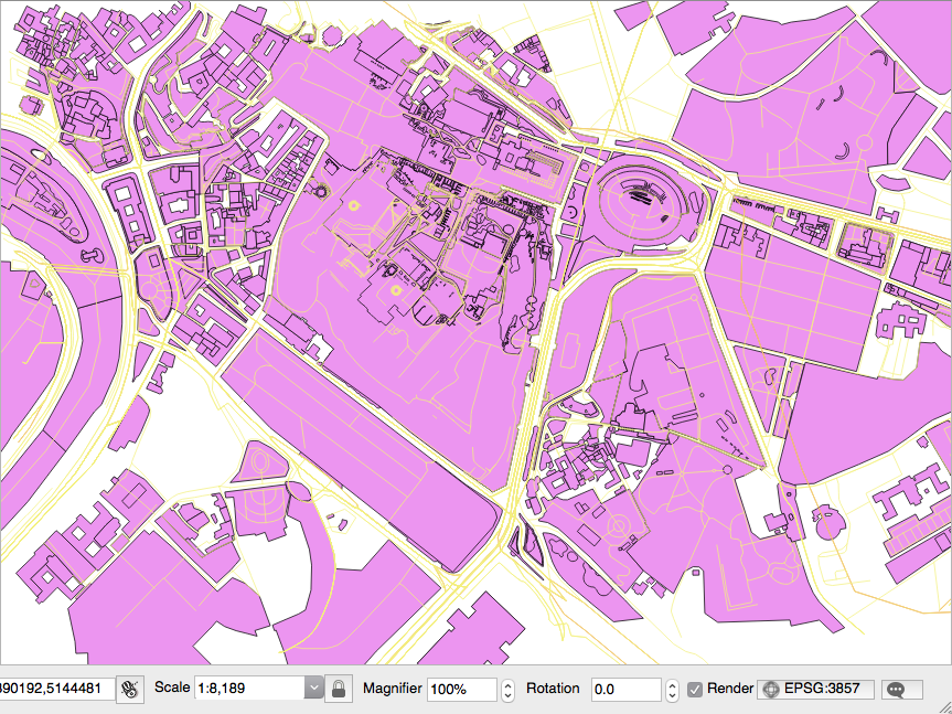
You can also try to open the virtual layer with a desktop GIS supporting a GDAL/OGR virtual driver such as Quantum GIS (QGIS). In the following screenshot, the Global_24h layer is displayed together with the shapefile of the countries that you can find in the dataset directory of the book:
      $ ogr2ogr -f PostgreSQL -t_srs EPSG:3857
      PG:"dbname='postgis_cookbook' user='me' password='mypassword'"
      -lco SCHEMA=chp01 global_24h.vrt -where "satellite='T'"
      -lco GEOMETRY_NAME=the_geom
      $ pg_dump -t chp01.global_24h --schema-only -U me postgis_cookbook

      CREATE TABLE global_24h (
        ogc_fid integer NOT NULL,
        latitude character varying,
        longitude character varying,
        brightness character varying,
        scan character varying,
        track character varying,
        acq_date character varying,
        acq_time character varying,
        satellite character varying,
        confidence character varying,
        version character varying,
        bright_t31 character varying,
        frp character varying,
        the_geom public.geometry(Point,3857)
      );
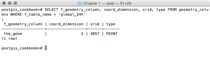
      postgis_cookbook=# SELECT f_geometry_column, coord_dimension,
      srid, type FROM geometry_columns
      WHERE f_table_name = 'global_24h';
The output of the preceding command is as follows:
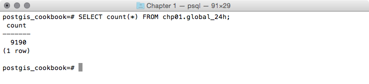
postgis_cookbook=# SELECT count(*) FROM chp01.global_24h;
The output of the preceding command is as follows:
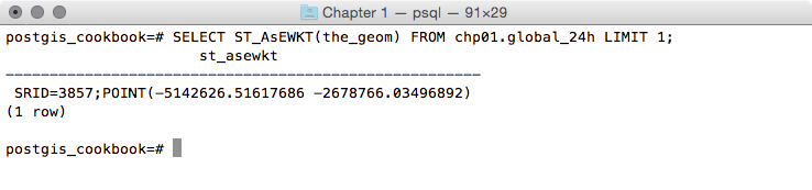
      postgis_cookbook=# SELECT ST_AsEWKT(the_geom)
      FROM chp01.global_24h LIMIT 1;
The output of the preceding command is as follows:
As mentioned in the GDAL documentation:
GDAL supports the reading and writing of nonspatial tabular data stored as a CSV file, but we need to use a virtual format to derive the geometry of the layers from attribute columns in the CSV file (the longitude and latitude coordinates for each point). For this purpose, you need to at least specify in the driver the path to the CSV file (the SrcDataSource element), the geometry type (the GeometryType element), the spatial reference definition for the layer (the LayerSRS element), and the way the driver can derive the geometric information (the GeometryField element).
There are many other options and reasons for using OGR virtual formats; if you are interested in developing a better understanding, please refer to the GDAL documentation available at http://www.gdal.org/drv_vrt.html.
After a virtual format is correctly created, the original flat nonspatial dataset is spatially supported by GDAL and software-based on GDAL. This is the reason why we can manipulate these files with GDAL commands such as ogrinfo and ogr2ogr, and with desktop GIS software such as QGIS.
Once we have verified that GDAL can correctly read the features from the virtual driver, we can easily import them in PostGIS using the popular ogr2ogr command-line utility. The ogr2ogr command has a plethora of options, so refer to its documentation at http://www.gdal.org/ogr2ogr.html for a more in-depth discussion.
In this recipe, you have just seen some of these options, such as:
If you need to import a shapefile in PostGIS, you have at least a couple of options such as the ogr2ogr GDAL command, as you have seen previously, or the shp2pgsql PostGIS command.
In this recipe, you will load a shapefile in the database using the shp2pgsql command, analyze it with the ogrinfo command, and display it in QGIS desktop software.
The steps you need to follow to complete this recipe are as follows:
$ ogr2ogr global_24h.shp global_24h.vrt
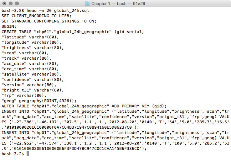
      $ shp2pgsql -G -I global_24h.shp
        chp01.global_24h_geographic > global_24h.sql
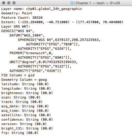
$ head -n 20 global_24h.sql
The output of the preceding command is as follows:
$ psql -U me -d postgis_cookbook -f global_24h.sql
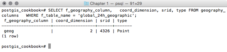
      postgis_cookbook=# SELECT f_geography_column,   coord_dimension,
      srid, type FROM geography_columns
      WHERE f_table_name = 'global_24h_geographic';
The output of the preceding command is as follows:
      $ ogrinfo PG:"dbname='postgis_cookbook' user='me'
        password='mypassword'" chp01.global_24h_geographic -fid 1
The output of the preceding command is as follows:
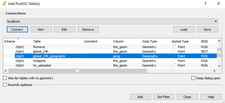
Now, open QGIS and try to add the new layer to the map. Navigate to Layer | Add Layer | Add PostGIS layers and provide the connection information, and then add the layer to the map as shown in the following screenshot:
The PostGIS command, shp2pgsql, allows the user to import a shapefile in the PostGIS database. Basically, it generates a PostgreSQL dump file that can be used to load data by running it from within PostgreSQL.
The SQL file will be generally composed of the following sections:
To get a complete list of the shp2pgsql command options and their meanings, just type the command name in the shell (or in the command prompt, if you are on Windows) and check the output.
There are GUI tools to manage data in and out of PostGIS, generally integrated into GIS desktop software such as QGIS. In the last chapter of this book, we will take a look at the most popular one.
In this recipe, you will use the popular ogr2ogr GDAL command for importing and exporting vector data from PostGIS.
Firstly, you will import a shapefile in PostGIS using the most significant options of the ogr2ogr command. Then, still using ogr2ogr, you will export the results of a spatial query performed in PostGIS to a couple of GDAL-supported vector formats.
The steps you need to follow to complete this recipe are as follows:
      $ ogr2ogr -f PostgreSQL -sql "SELECT ISO2,
      NAME AS country_name FROM wborders WHERE REGION=2" -nlt
      MULTIPOLYGON PG:"dbname='postgis_cookbook' user='me'
      password='mypassword'" -nln africa_countries
      -lco SCHEMA=chp01 -lco GEOMETRY_NAME=the_geom wborders.shp
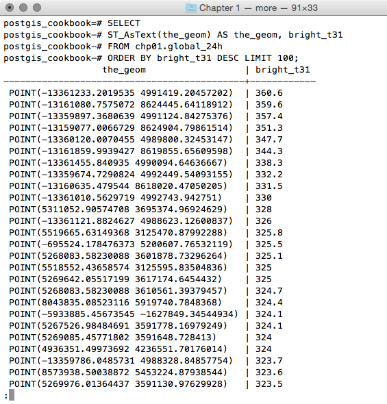
      postgis_cookbook=# SELECTST_AsText(the_geom) AS the_geom, bright_t31
      FROM chp01.global_24h
      ORDER BY bright_t31 DESC LIMIT 100;
The output of the preceding command is as follows:
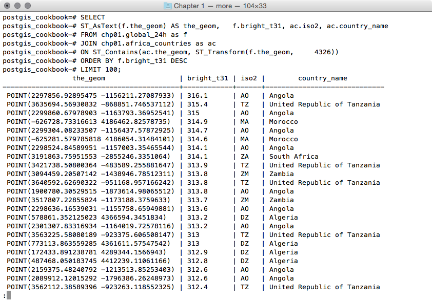
      postgis_cookbook=# SELECT ST_AsText(f.the_geom)
      AS the_geom, f.bright_t31, ac.iso2, ac.country_name
      FROM chp01.global_24h as f
      JOIN chp01.africa_countries as ac
      ON ST_Contains(ac.the_geom, ST_Transform(f.the_geom, 4326))
      ORDER BY f.bright_t31 DESCLIMIT 100;
The output of the preceding command is as follows:
You will now export the result of this query to a vector format supported by GDAL, such as GeoJSON, in the WGS 84 spatial reference using ogr2ogr:
      $ ogr2ogr -f GeoJSON -t_srs EPSG:4326 warmest_hs.geojson
      PG:"dbname='postgis_cookbook' user='me' password='mypassword'" -sql "
      SELECT f.the_geom as the_geom, f.bright_t31,
             ac.iso2, ac.country_name
      FROM chp01.global_24h as f JOIN chp01.africa_countries as ac
      ON ST_Contains(ac.the_geom, ST_Transform(f.the_geom, 4326))
      ORDER BY f.bright_t31 DESC LIMIT 100"
      $ ogr2ogr -t_srs EPSG:4326 -f CSV -lco GEOMETRY=AS_XY
      -lco SEPARATOR=TAB warmest_hs.csv PG:"dbname='postgis_cookbook'
       user='me' password='mypassword'" -sql "
       SELECT f.the_geom, f.bright_t31,
         ac.iso2, ac.country_name
       FROM chp01.global_24h as f JOIN chp01.africa_countries as ac
       ON ST_Contains(ac.the_geom, ST_Transform(f.the_geom, 4326))
       ORDER BY f.bright_t31 DESC  LIMIT 100"
GDAL is an open source library that comes together with several command-line utilities, which let the user translate and process raster and vector geodatasets into a plethora of formats. In the case of vector datasets, there is a GDAL sublibrary for managing vector datasets named OGR (therefore, when talking about vector datasets in the context of GDAL, we can also use the expression OGR dataset).
When you are working with an OGR dataset, two of the most popular OGR commands are ogrinfo, which lists many kinds of information from an OGR dataset, and ogr2ogr, which converts the OGR dataset from one format to another.
It is possible to retrieve a list of the supported OGR vector formats using the -formats option on any OGR commands, for example, with ogr2ogr:
$ ogr2ogr --formats
The output of the preceding command is as follows:
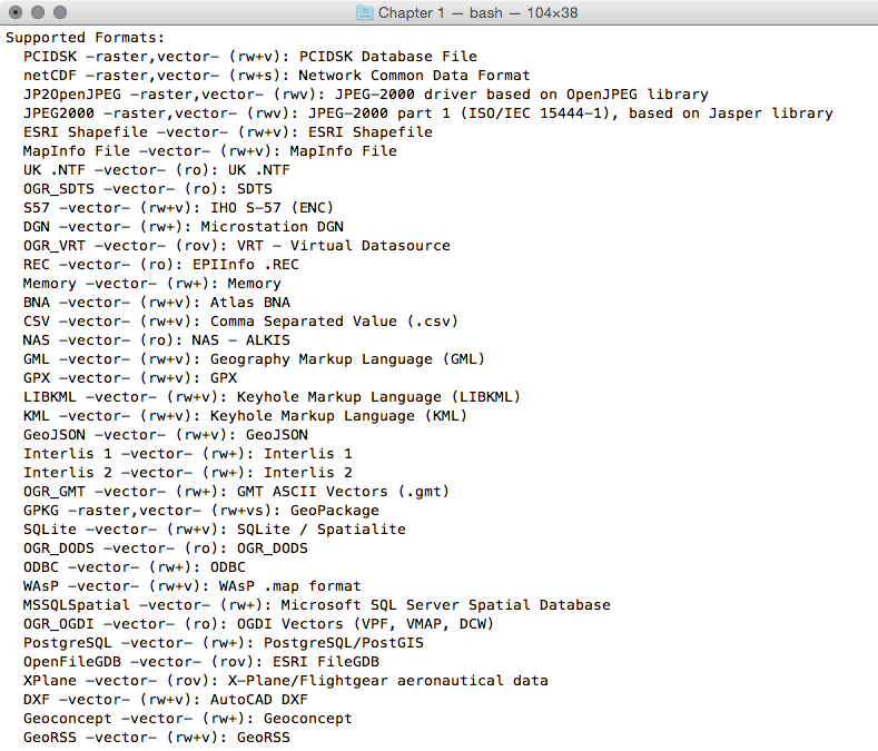
Note that some formats are read-only, while others are read/write.
PostGIS is one of the supported read/write OGR formats, so it is possible to use the OGR API or any OGR commands (such as ogrinfo and ogr2ogr) to manipulate its datasets.
The ogr2ogr command has many options and parameters; in this recipe, you have seen some of the most notable ones such as -f to define the output format, -t_srs to reproject/transform the dataset, and -sql to define an (eventually spatial) query in the input OGR dataset.
When using ogrinfo and ogr2ogr together with the desired option and parameters, you have to define the datasets. When specifying a PostGIS dataset, you need a connection string that is defined as follows:
PG:"dbname='postgis_cookbook' user='me' password='mypassword'"
You can find more information about the ogrinfo and ogr2ogr commands on the GDAL website available at http://www.gdal.org.
If you need more information about the PostGIS driver, you should check its related documentation page available at http://www.gdal.org/drv_pg.html.
In many GIS workflows, there is a typical scenario where subsets of a PostGIS table must be deployed to external users in a filesystem format (most typically, shapefiles or a spatialite database). Often, there is also the reverse process, where datasets received from different users have to be uploaded to the PostGIS database.
In this recipe, we will simulate both of these data flows. You will first create the data flow for processing the shapefiles out of PostGIS, and then the reverse data flow for uploading the shapefiles.
You will do it using the power of bash scripting and the ogr2ogr command.
If you didn't follow all the other recipes, be sure to import the hotspots (Global_24h.csv) and the countries dataset (countries.shp) in PostGIS. The following is how to do it with ogr2ogr (you should import both the datasets in their original SRID, 4326, to make spatial operations faster):
      $ ogr2ogr -f PostgreSQL PG:"dbname='postgis_cookbook'
      user='me' password='mypassword'" -lco SCHEMA=chp01 global_24h.vrt
      -lco OVERWRITE=YES -lco GEOMETRY_NAME=the_geom -nln hotspots
      $ ogr2ogr -f PostgreSQL -sql "SELECT ISO2, NAME AS country_name
      FROM wborders" -nlt MULTIPOLYGON PG:"dbname='postgis_cookbook'
      user='me' password='mypassword'" -nln countries
      -lco SCHEMA=chp01 -lco OVERWRITE=YES
      -lco GEOMETRY_NAME=the_geom wborders.shp
The steps you need to follow to complete this recipe are as follows:
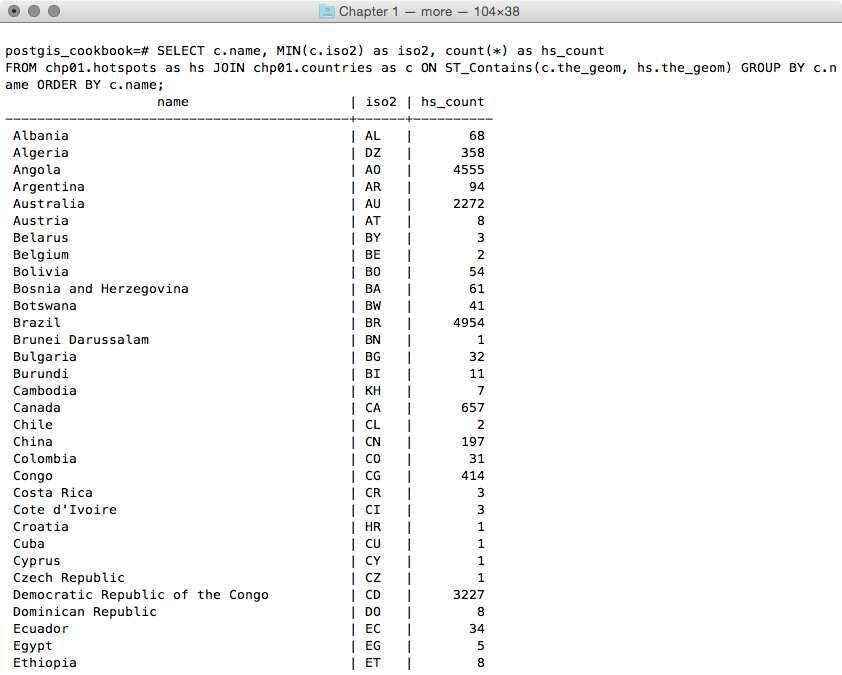
      postgis_cookbook=> SELECT c.country_name, MIN(c.iso2)
      as iso2, count(*) as hs_count FROM chp01.hotspots as hs
      JOIN chp01.countries as c ON ST_Contains(c.the_geom, hs.the_geom)
      GROUP BY c.country_name ORDER BY c.country_name;
The output of the preceding command is as follows:
      $ ogr2ogr -f CSV hs_countries.csv
      PG:"dbname='postgis_cookbook' user='me' password='mypassword'"
      -lco SCHEMA=chp01 -sql "SELECT c.country_name, MIN(c.iso2) as iso2,
      count(*) as hs_count FROM chp01.hotspots as hs
      JOIN chp01.countries as c ON ST_Contains(c.the_geom, hs.the_geom)
      GROUP BY c.country_name ORDER BY c.country_name"
      postgis_cookbook=> COPY (SELECT c.country_name, MIN(c.iso2) as iso2,
      count(*) as hs_count  FROM chp01.hotspots as hs
      JOIN chp01.countries as c  ON ST_Contains(c.the_geom, hs.the_geom)
      GROUP BY c.country_name  ORDER BY c.country_name)
      TO '/tmp/hs_countries.csv' WITH CSV HEADER;
#!/bin/bash
while IFS="," read country iso2 hs_count
do
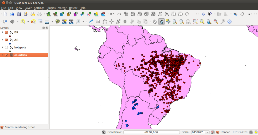
echo "Generating shapefile $iso2.shp for country
$country ($iso2) containing $hs_count features."
ogr2ogr out_shapefiles/$iso2.shp
PG:"dbname='postgis_cookbook' user='me' password='mypassword'"
-lco SCHEMA=chp01 -sql "SELECT ST_Transform(hs.the_geom, 4326),
hs.acq_date, hs.acq_time, hs.bright_t31
FROM chp01.hotspots as hs JOIN chp01.countries as c
ON ST_Contains(c.the_geom, ST_Transform(hs.the_geom, 4326))
WHERE c.iso2 = '$iso2'" done < hs_countries.csv
      chmod 775 export_shapefiles.sh
      mkdir out_shapefiles
      $ ./export_shapefiles.sh
      Generating shapefile AL.shp for country
        Albania (AL) containing 66 features.
      Generating shapefile DZ.shp for country
        Algeria (DZ) containing 361 features.
      ...
      Generating shapefile ZM.shp for country
        Zambia (ZM) containing 1575 features.
      Generating shapefile ZW.shp for country
        Zimbabwe (ZW) containing 179 features.
        @echo off
        for /f "tokens=1-3 delims=, skip=1" %%a in (hs_countries.csv) do (
          echo "Generating shapefile %%b.shp for country %%a
                (%%b) containing %%c features"
          ogr2ogr .\out_shapefiles\%%b.shp
          PG:"dbname='postgis_cookbook' user='me' password='mypassword'"
          -lco SCHEMA=chp01 -sql "SELECT ST_Transform(hs.the_geom, 4326),
          hs.acq_date, hs.acq_time, hs.bright_t31
          FROM chp01.hotspots as hs JOIN chp01.countries as c
          ON ST_Contains(c.the_geom, ST_Transform(hs.the_geom, 4326))
          WHERE c.iso2 = '%%b'"
        )
      >mkdir out_shapefiles
      >export_shapefiles.bat
      "Generating shapefile AL.shp for country
       Albania (AL) containing 66 features"
      "Generating shapefile DZ.shp for country
       Algeria (DZ) containing 361 features"
      ...
      "Generating shapefile ZW.shp for country
       Zimbabwe (ZW) containing 179 features"
      postgis_cookbook=# CREATE TABLE chp01.hs_uploaded
      (
        ogc_fid serial NOT NULL,
        acq_date character varying(80),
        acq_time character varying(80),
        bright_t31 character varying(80),
        iso2 character varying,
        upload_datetime character varying,
        shapefile character varying,
        the_geom geometry(POINT, 4326),
        CONSTRAINT hs_uploaded_pk PRIMARY KEY (ogc_fid)
      );
$ brew install findutils
        #!/bin/bash
        for f in `find out_shapefiles -name \*.shp -printf "%f\n"`
        do
          echo "Importing shapefile $f to chp01.hs_uploaded PostGIS
            table..." #, ${f%.*}"
          ogr2ogr -append -update  -f PostgreSQL
          PG:"dbname='postgis_cookbook' user='me'
          password='mypassword'" out_shapefiles/$f
          -nln chp01.hs_uploaded -sql "SELECT acq_date, acq_time,
          bright_t31, '${f%.*}' AS iso2, '`date`' AS upload_datetime,
         'out_shapefiles/$f' as shapefile FROM ${f%.*}"
        done
      $ chmod 775 import_shapefiles.sh
      $ ./import_shapefiles.sh
      Importing shapefile DO.shp to chp01.hs_uploaded PostGIS table
      ...
      Importing shapefile ID.shp to chp01.hs_uploaded PostGIS table
      ...
      Importing shapefile AR.shp to chp01.hs_uploaded PostGIS table
      ......
Now, go to step 14.
        @echo off
        for %%I in (out_shapefiles\*.shp*) do (
          echo Importing shapefile %%~nxI to chp01.hs_uploaded
          PostGIS table...

          ogr2ogr -append -update  -f PostgreSQL
          PG:"dbname='postgis_cookbook' user='me'
          password='password'" out_shapefiles/%%~nxI
          -nln chp01.hs_uploaded -sql "SELECT acq_date, acq_time,
          bright_t31, '%%~nI' AS iso2, '%date%' AS upload_datetime,
          'out_shapefiles/%%~nxI' as shapefile FROM %%~nI"
        )
      >import_shapefiles.bat
      Importing shapefile AL.shp to chp01.hs_uploaded PostGIS table...
      Importing shapefile AO.shp to chp01.hs_uploaded PostGIS table...
      Importing shapefile AR.shp to chp01.hs_uploaded PostGIS table......
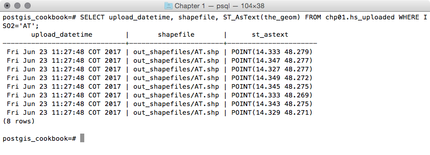
      postgis_cookbook=# SELECT upload_datetime,
      shapefile, ST_AsText(wkb_geometry)
      FROM chp01.hs_uploaded WHERE ISO2='AT';
The output of the preceding command is as follows:
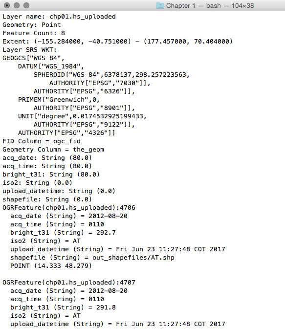
      $ ogrinfo PG:"dbname='postgis_cookbook' user='me'
      password='mypassword'"
      chp01.hs_uploaded -where "iso2='AT'"
The output of the preceding command is as follows:
You could implement both the data flows (processing shapefiles out from PostGIS, and then into it again) thanks to the power of the ogr2ogr GDAL command.
You have been using this command in different forms and with the most important input parameters in other recipes, so you should now have a good understanding of it.
Here, it is worth mentioning the way OGR lets you export the information related to the current datetime and the original shapefile name to the PostGIS table. Inside the import_shapefiles.sh (Linux, OS X) or the import_shapefiles.bat (Windows) scripts, the core is the line with the ogr2ogr command (here is the Linux version):
ogr2ogr -append -update -f PostgreSQL PG:"dbname='postgis_cookbook' user='me' password='mypassword'" out_shapefiles/$f -nln chp01.hs_uploaded -sql "SELECT acq_date, acq_time, bright_t31, '${f%.*}' AS iso2, '`date`' AS upload_datetime, 'out_shapefiles/$f' as shapefile FROM ${f%.*}"
Thanks to the -sql option, you can specify the two additional fields, getting their values from the system date command and the filename that is being iterated from the script.
In this recipe, you will export a PostGIS table to a shapefile using the pgsql2shp command that is shipped with any PostGIS distribution.
The steps you need to follow to complete this recipe are as follows:
      $ shp2pgsql -I -d -s 4326 -W LATIN1 -g the_geom countries.shp
      chp01.countries > countries.sql
      $ psql -U me -d postgis_cookbook -f countries.sql
      $ ogr2ogr -f PostgreSQL PG:"dbname='postgis_cookbook' user='me'
      password='mypassword'"
      -lco SCHEMA=chp01 countries.shp -nlt MULTIPOLYGON -lco OVERWRITE=YES
      -lco GEOMETRY_NAME=the_geom
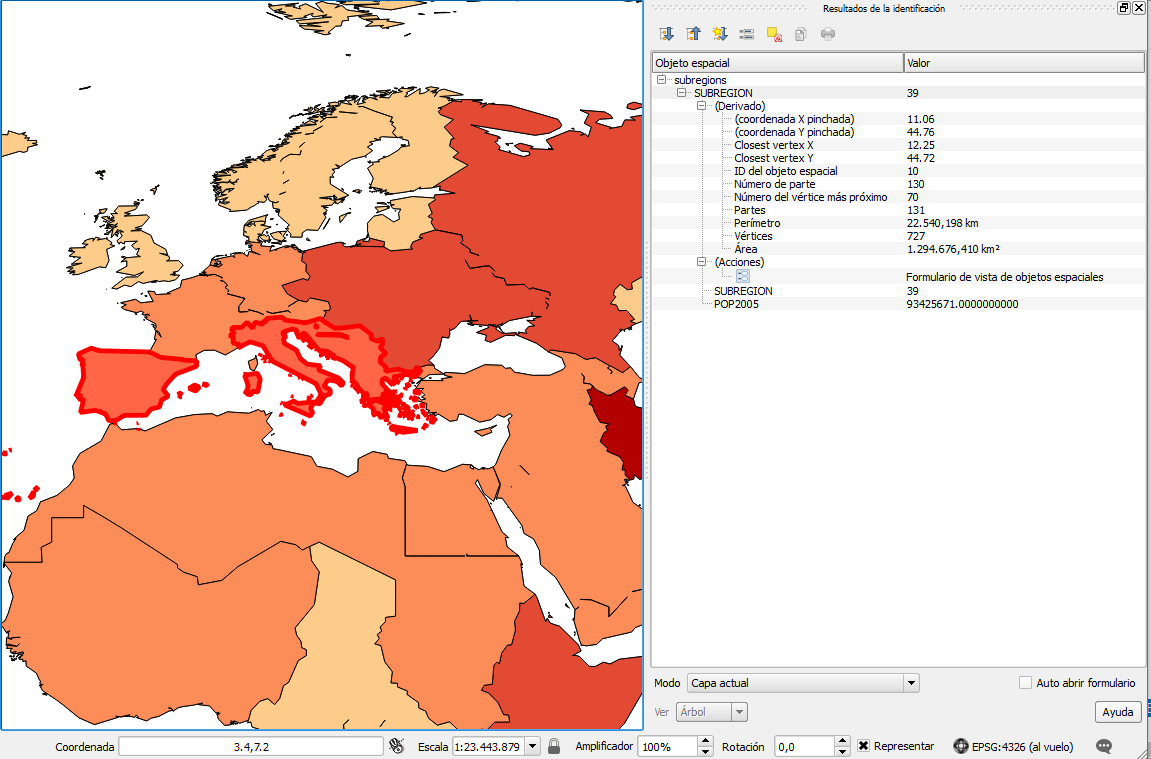
      postgis_cookbook=> SELECT subregion,
        ST_Union(the_geom) AS the_geom, SUM(pop2005) AS pop2005
        FROM chp01.countries GROUP BY subregion;
      $ pgsql2shp -f subregions.shp -h localhost -u me -P mypassword
      postgis_cookbook "SELECT MIN(subregion) AS subregion,
      ST_Union(the_geom) AS the_geom, SUM(pop2005) AS pop2005
      FROM chp01.countries GROUP BY subregion;"

      Initializing...
      Done (postgis major version: 2).
      Output shape: Polygon
      Dumping: X [23 rows].
You have exported the results of a spatial query to a shapefile using the pgsql2shp PostGIS command. The spatial query you have used aggregates fields using the SUM PostgreSQL function for summing country populations in the same subregion, and the ST_Union PostGIS function to aggregate the corresponding geometries as a geometric union.
The pgsql2shp command allows you to export PostGIS tables and queries to shapefiles. The options you need to specify are quite similar to the ones you use to connect to PostgreSQL with psql. To get a full list of these options, just type pgsql2shp in your command prompt and read the output.
In this recipe, you will import OpenStreetMap (OSM) data to PostGIS using the osm2pgsql command.
You will first download a sample dataset from the OSM website, and then you will import it using the osm2pgsql command.
You will add the imported layers in GIS desktop software and generate a view to get subdatasets, using the hstore PostgreSQL additional module to extract features based on their tags.
We need the following in place before we can proceed with the steps required for the recipe:
$ sudo apt-get install osm2pgsql
$ osm2pgsqlosm2pgsql SVN version 0.80.0 (32bit id space)
      postgres=# CREATE DATABASE rome OWNER me;
      postgres=# \connect rome;
      rome=# create extension postgis;
      $ sudo apt-get update
      $ sudo apt-get install postgresql-contrib-9.6
      $ psql -U me -d romerome=# CREATE EXTENSION hstore;
The steps you need to follow to complete this recipe are as follows:
      $ osm2pgsql -d rome -U me --hstore map.osm
      osm2pgsql SVN version 0.80.0 (32bit id space)Using projection
      SRS 900913 (Spherical Mercator)Setting up table:
      planet_osm_point...All indexes on planet_osm_polygon created
      in 1sCompleted planet_osm_polygonOsm2pgsql took 3s overall
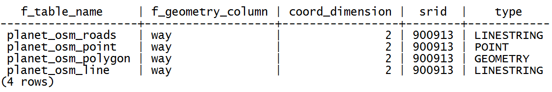
      rome=# SELECT f_table_name, f_geometry_column,
      coord_dimension, srid, type FROM geometry_columns;
The output of the preceding command is shown here:
      rome=# CREATE VIEW rome_trees AS SELECT way, tags
      FROM planet_osm_polygon WHERE (tags -> 'landcover') = 'trees';
OpenStreetMap is a popular collaborative project for creating a free map of the world. Every user participating in the project can edit data; at the same time, it is possible for everyone to download those datasets in .osm datafiles (an XML format) under the terms of the Open Data Commons Open Database License (ODbL) at the time of writing.
The osm2pgsql command is a command-line tool that can import .osm datafiles (eventually zipped) to the PostGIS database. To use the command, it is enough to give the PostgreSQL connection parameters and the .osm file to import.
It is possible to import only features that have certain tags in the spatial database, as defined in the default.style configuration file. You can decide to comment in or out the OSM tagged features that you would like to import, or not, from this file. The command by default exports all the nodes and ways to linestring, point, and geometry PostGIS geometries.
It is highly recommended to enable hstore support in the PostgreSQL database and use the -hstore option of osm2pgsql when importing the data. Having enabled this support, the OSM tags for each feature will be stored in a hstore PostgreSQL data type, which is optimized for storing (and retrieving) sets of key/values pairs in a single field. This way, it will be possible to query the database as follows:
SELECT way, tags FROM planet_osm_polygon WHERE (tags -> 'landcover') = 'trees';
PostGIS 2.0 now has full support for raster datasets, and it is possible to import raster datasets using the raster2pgsql command.
In this recipe, you will import a raster file to PostGIS using the raster2pgsql command. This command, included in any PostGIS distribution from version 2.0 onward, is able to generate an SQL dump to be loaded in PostGIS for any GDAL raster-supported format (in the same fashion that the shp2pgsql command does for shapefiles).
After loading the raster to PostGIS, you will inspect it both with SQL commands (analyzing the raster metadata information contained in the database), and with the gdalinfo command-line utility (to understand the way the input raster2pgsql parameters have been reflected in the PostGIS import process).
You will finally open the raster in a desktop GIS and try a basic spatial query, mixing vector and raster tables.
We need the following in place before we can proceed with the steps required for the recipe:
      $ shp2pgsql -I -d -s 4326 -W LATIN1 -g the_geom countries.shp
      chp01.countries > countries.sql
      $ psql -U me -d postgis_cookbook -f countries.sql
The steps you need to follow to complete this recipe are as follows:
      $ gdalinfo worldclim/tmax09.bil

      Driver: EHdr/ESRI .hdr Labelled
      Files: worldclim/tmax9.bil
             worldclim/tmax9.hdr
      Size is 2160, 900
      Coordinate System is:
      GEOGCS[""WGS 84"",
        DATUM[""WGS_1984"",
          SPHEROID[""WGS 84"",6378137,298.257223563,
            AUTHORITY[""EPSG"",""7030""]],
          TOWGS84[0,0,0,0,0,0,0],
          AUTHORITY[""EPSG"",""6326""]],
        PRIMEM[""Greenwich"",0,
          AUTHORITY[""EPSG"",""8901""]],
        UNIT[""degree"",0.0174532925199433,
        AUTHORITY[""EPSG"",""9108""]],
      AUTHORITY[""EPSG"",""4326""]]
      Origin = (-180.000000000000057,90.000000000000000)
      Pixel Size = (0.166666666666667,-0.166666666666667)
      Corner Coordinates:
        Upper Left (-180.0000000, 90.0000000) (180d 0'' 0.00""W, 90d
                                               0'' 0.00""N)
        Lower Left (-180.0000000, -60.0000000) (180d 0'' 0.00""W, 60d
                                                0'' 0.00""S)
        Upper Right ( 180.0000000, 90.0000000) (180d 0'' 0.00""E, 90d
                                                0'' 0.00""N)
        Lower Right ( 180.0000000, -60.0000000) (180d 0'' 0.00""E, 60d
                                                 0'' 0.00""S)
        Center ( 0.0000000, 15.0000000) ( 0d 0'' 0.00""E, 15d
                                          0'' 0.00""N)
        Band 1 Block=2160x1 Type=Int16, ColorInterp=Undefined
        Min=-153.000 Max=441.000
        NoData Value=-9999
      $ raster2pgsql -I -C -F -t 100x100 -s 4326
      worldclim/tmax01.bil chp01.tmax01 > tmax01.sql
      $ psql -d postgis_cookbook -U me -f tmax01.sql
If you are in Linux, you may pipe the two commands in a unique line:
      $ raster2pgsql -I -C -M -F -t 100x100 worldclim/tmax01.bil
      chp01.tmax01 | psql -d postgis_cookbook -U me -f tmax01.sql
      $ pg_dump -t chp01.tmax01 --schema-only -U me postgis_cookbook
      ...
      CREATE TABLE tmax01 (
        rid integer NOT NULL,
        rast public.raster,
        filename text,
        CONSTRAINT enforce_height_rast CHECK (
          (public.st_height(rast) = 100)
        ),
        CONSTRAINT enforce_max_extent_rast CHECK (public.st_coveredby
          (public.st_convexhull(rast), ''0103...''::public.geometry)
        ),
        CONSTRAINT enforce_nodata_values_rast CHECK (
          ((public._raster_constraint_nodata_values(rast)
            )::numeric(16,10)[] = ''{0}''::numeric(16,10)[])
          ),
        CONSTRAINT enforce_num_bands_rast CHECK (
          (public.st_numbands(rast) = 1)
        ),
        CONSTRAINT enforce_out_db_rast CHECK (
          (public._raster_constraint_out_db(rast) = ''{f}''::boolean[])
          ),
        CONSTRAINT enforce_pixel_types_rast CHECK (
          (public._raster_constraint_pixel_types(rast) =
           ''{16BUI}''::text[])
          ),
        CONSTRAINT enforce_same_alignment_rast CHECK (
          (public.st_samealignment(rast, ''01000...''::public.raster)
        ),
        CONSTRAINT enforce_scalex_rast CHECK (
          ((public.st_scalex(rast))::numeric(16,10) =
            0.166666666666667::numeric(16,10))
           ),
        CONSTRAINT enforce_scaley_rast CHECK (
          ((public.st_scaley(rast))::numeric(16,10) =
            (-0.166666666666667)::numeric(16,10))
          ),
        CONSTRAINT enforce_srid_rast CHECK ((public.st_srid(rast) = 0)),
        CONSTRAINT enforce_width_rast CHECK ((public.st_width(rast) = 100))
      );
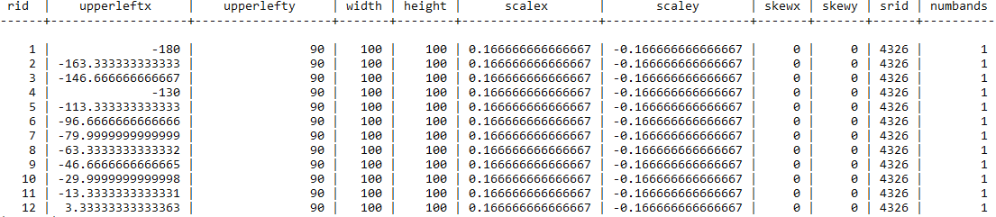
postgis_cookbook=# SELECT * FROM raster_columns;
postgis_cookbook=# SELECT count(*) FROM chp01.tmax01;
The output of the preceding command is as follows:
      count
      -------
      198
      (1 row)
      gdalinfo PG":host=localhost port=5432 dbname=postgis_cookbook
      user=me password=mypassword schema='chp01' table='tmax01'"
      gdalinfo PG":host=localhost port=5432 dbname=postgis_cookbook
      user=me password=mypassword schema='chp01' table='tmax01' mode=2"
      $ ogr2ogr temp_grid.shp PG:"host=localhost port=5432
      dbname='postgis_cookbook' user='me' password='mypassword'"
      -sql "SELECT rid, filename, ST_Envelope(rast) as the_geom
      FROM chp01.tmax01"
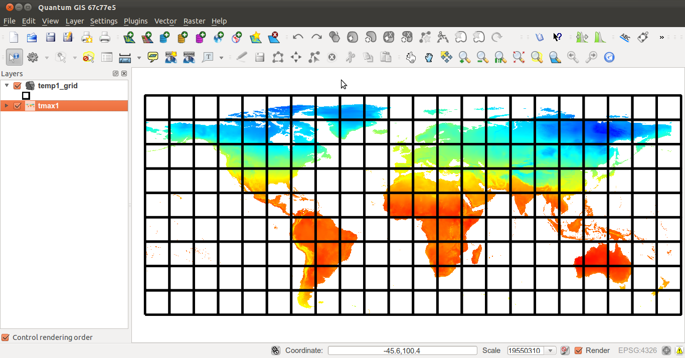
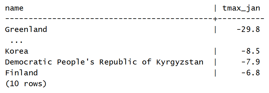
      SELECT * FROM (
        SELECT c.name, ST_Value(t.rast,
          ST_Centroid(c.the_geom))/10 as tmax_jan FROM chp01.tmax01 AS t
        JOIN chp01.countries AS c
        ON ST_Intersects(t.rast, ST_Centroid(c.the_geom))
      ) AS foo
      ORDER BY tmax_jan LIMIT 10;
The output is as follows:
The raster2pgsql command is able to load any raster formats supported by GDAL in PostGIS. You can have a format list supported by your GDAL installation by typing the following command:
$ gdalinfo --formats
In this recipe, you have been importing one raster file using some of the most common raster2pgsql options:
$ raster2pgsql -I -C -F -t 100x100 -s 4326 worldclim/tmax01.bil chp01.tmax01 > tmax01.sql
The -I option creates a GIST spatial index for the raster column. The -C option will create the standard set of constraints after the rasters have been loaded. The -F option will add a column with the filename of the raster that has been loaded. This is useful when you are appending many raster files to the same PostGIS raster table. The -s option sets the raster's SRID.
If you decide to include the -t option, then you will cut the original raster into tiles, each inserted as a single row in the raster table. In this case, you decided to cut the raster into 100 x 100 tiles, resulting in 198 table rows in the raster table.
Another important option is -R, which will register the raster as out-of-db; in such a case, only the metadata will be inserted in the database, while the raster will be out of the database.
The raster table contains an identifier for each row, the raster itself (eventually one of its tiles, if using the -t option), and eventually the original filename, if you used the -F option, as in this case.
You can analyze the PostGIS raster using SQL commands or the gdalinfo command. Using SQL, you can query the raster_columns view to get the most significant raster metadata (spatial reference, band number, scale, block size, and so on).
With gdalinfo, you can access the same information, using a connection string with the following syntax:
gdalinfo PG":host=localhost port=5432 dbname=postgis_cookbook user=me password=mypassword schema='chp01' table='tmax01' mode=2"
The mode parameter is not influential if you loaded the whole raster as a single block (for example, if you did not specify the -t option). But, as in the use case of this recipe, if you split it into tiles, gdalinfo will see each tile as a single subdataset with the default behavior (mode=1). If you want GDAL to consider the raster table as a unique raster dataset, you have to specify the mode option and explicitly set it to 2.
This recipe will guide you through the importing of multiple rasters at a time.
You will first import some different single band rasters to a unique single band raster table using the raster2pgsql command.
Then, you will try an alternative approach, merging the original single band rasters in a virtual raster, with one band for each of the original rasters, and then load the multiband raster to a raster table. To accomplish this, you will use the GDAL gdalbuildvrt command and then load the data to PostGIS with raster2pgsql.
Be sure to have all the original raster datasets you have been using for the previous recipe.
The steps you need to follow to complete this recipe are as follows:
      $ raster2pgsql -d -I -C -M -F -t 100x100 -s 4326
      worldclim/tmax*.bil chp01.tmax_2012 > tmax_2012.sql
      $ psql -d postgis_cookbook -U me -f tmax_2012.sql
      postgis_cookbook=# SELECT r_raster_column, srid,
      ROUND(scale_x::numeric, 2) AS scale_x,
      ROUND(scale_y::numeric, 2) AS scale_y, blocksize_x,
      blocksize_y, num_bands, pixel_types, nodata_values, out_db
      FROM raster_columns where r_table_schema='chp01'
      AND r_table_name ='tmax_2012';

      SELECT rid, (foo.md).*
      FROM (SELECT rid, ST_MetaData(rast) As md
      FROM chp01.tmax_2012) As foo;
The output of the preceding command is as shown here:
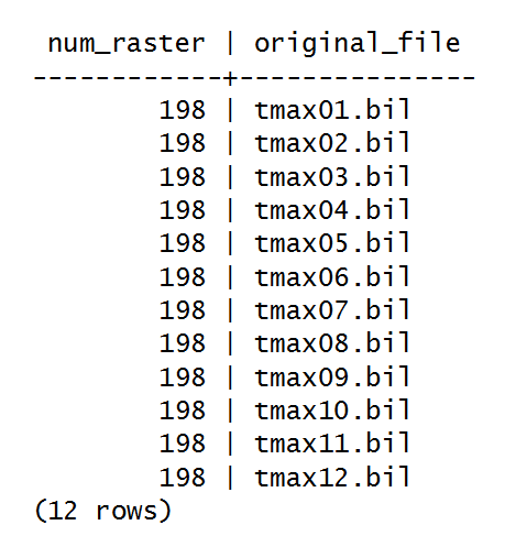
If you now query the table, you would be able to derive the month for each raster row only from the original_file column. In the table, you have imported 198 distinct records (rasters) for each of the 12 original files (we divided them into 100 x 100 blocks, if you remember). Test this with the following query:
      postgis_cookbook=# SELECT COUNT(*) AS num_raster,
      MIN(filename) as original_file FROM chp01.tmax_2012
      GROUP BY filename ORDER BY filename;
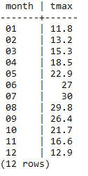
      SELECT REPLACE(REPLACE(filename, 'tmax', ''), '.bil', '') AS month,
      (ST_VALUE(rast, ST_SetSRID(ST_Point(12.49, 41.88), 4326))/10) AS tmax
      FROM chp01.tmax_2012
      WHERE rid IN (
        SELECT rid FROM chp01.tmax_2012
        WHERE ST_Intersects(ST_Envelope(rast),
              ST_SetSRID(ST_Point(12.49, 41.88), 4326))
      )
      ORDER BY month;
The output of the preceding command is as shown here:
$ gdalbuildvrt -separate tmax_2012.vrt worldclim/tmax*.bil
      <VRTDataset rasterXSize="2160" rasterYSize="900">
        <SRS>GEOGCS...</SRS>
        <GeoTransform>
          -1.8000000000000006e+02, 1.6666666666666699e-01, ...
        </GeoTransform>
        <VRTRasterBand dataType="Int16" band="1">
          <NoDataValue>-9.99900000000000E+03</NoDataValue>
          <ComplexSource>
            <SourceFilename relativeToVRT="1">
              worldclim/tmax01.bil
            </SourceFilename>
            <SourceBand>1</SourceBand>
            <SourceProperties RasterXSize="2160" RasterYSize="900"
             DataType="Int16" BlockXSize="2160" BlockYSize="1" />
            <SrcRect xOff="0" yOff="0" xSize="2160" ySize="900" />
            <DstRect xOff="0" yOff="0" xSize="2160" ySize="900" />
            <NODATA>-9999</NODATA>
          </ComplexSource>
        </VRTRasterBand>
      <VRTRasterBand dataType="Int16" band="2">
      ...
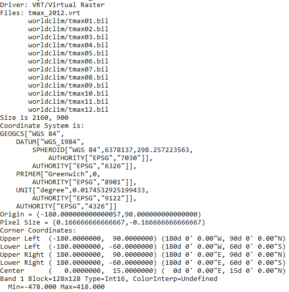
$ gdalinfo tmax_2012.vrt
The output of the preceding command is as follows:
 ...
...$ raster2pgsql -d -I -C -M -F -t 100x100 -s 4326 tmax_2012.vrt
chp01.tmax_2012_multi > tmax_2012_multi.sql
$ psql -d postgis_cookbook -U me -f tmax_2012_multi.sql
     postgis_cookbook=# SELECT r_raster_column, srid, blocksize_x,
     blocksize_y, num_bands, pixel_types
     from raster_columns where r_table_schema='chp01'
     AND r_table_name ='tmax_2012_multi';

      postgis_cookbook=# SELECT
      (ST_VALUE(rast, 1, ST_SetSRID(ST_Point(12.49, 41.88), 4326))/10)
      AS jan,
      (ST_VALUE(rast, 2, ST_SetSRID(ST_Point(12.49, 41.88), 4326))/10)
      AS feb,
      (ST_VALUE(rast, 3, ST_SetSRID(ST_Point(12.49, 41.88), 4326))/10)
      AS mar,
      (ST_VALUE(rast, 4, ST_SetSRID(ST_Point(12.49, 41.88), 4326))/10)
      AS apr,
      (ST_VALUE(rast, 5, ST_SetSRID(ST_Point(12.49, 41.88), 4326))/10)
      AS may,
      (ST_VALUE(rast, 6, ST_SetSRID(ST_Point(12.49, 41.88), 4326))/10)
      AS jun,
      (ST_VALUE(rast, 7, ST_SetSRID(ST_Point(12.49, 41.88), 4326))/10)
      AS jul,
      (ST_VALUE(rast, 8, ST_SetSRID(ST_Point(12.49, 41.88), 4326))/10)
      AS aug,
      (ST_VALUE(rast, 9, ST_SetSRID(ST_Point(12.49, 41.88), 4326))/10)
      AS sep,
      (ST_VALUE(rast, 10, ST_SetSRID(ST_Point(12.49, 41.88), 4326))/10)
      AS oct,
      (ST_VALUE(rast, 11, ST_SetSRID(ST_Point(12.49, 41.88), 4326))/10)
      AS nov,
      (ST_VALUE(rast, 12, ST_SetSRID(ST_Point(12.49, 41.88), 4326))/10)
      AS dec
      FROM chp01.tmax_2012_multi WHERE rid IN (
        SELECT rid FROM chp01.tmax_2012_multi
        WHERE ST_Intersects(rast, ST_SetSRID(ST_Point(12.49, 41.88), 4326))
      );
The output of the preceding command is as follows:

You can import raster datasets in PostGIS using the raster2pgsql command.
In a scenario where you have multiple rasters representing the same variable at different times, as in this recipe, it makes sense to store all of the original rasters as a single table in PostGIS. In this recipe, we have the same variable (average maximum temperature) represented by a single raster for each month. You have seen that you could proceed in two different ways:
In this recipe, you will see a couple of main options for exporting PostGIS rasters to different raster formats. They are both provided as command-line tools, gdal_translate and gdalwarp, by GDAL.
You need the following in place before you can proceed with the steps required for the recipe:
$ gdalinfo --formats | grep -i postgis
The output of the preceding command is as follows:
PostGISRaster (rw): PostGIS Raster driver
      $ gdalinfo PG:"host=localhost port=5432
      dbname='postgis_cookbook' user='me' password='mypassword'
      schema='chp01' table='tmax_2012_multi' mode='2'"
The steps you need to follow to complete this recipe are as follows:
      $ gdal_translate -b 1 -b 2 -b 3 -b 4 -b 5 -b 6
      PG:"host=localhost port=5432 dbname='postgis_cookbook'
      user='me' password='mypassword' schema='chp01'
      table='tmax_2012_multi' mode='2'" tmax_2012_multi_123456.tif
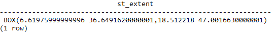
      postgis_cookbook=# SELECT ST_Extent(the_geom)
      FROM chp01.countries WHERE name = 'Italy';
The output of the preceding command is as follows:
      $ gdal_translate -projwin 6.619 47.095 18.515 36.649
      PG:"host=localhost port=5432 dbname='postgis_cookbook'
      user='me' password='mypassword' schema='chp01'
      table='tmax_2012_multi' mode='2'" tmax_2012_multi.tif
      gdalwarp -t_srs EPSG:3857 PG:"host=localhost port=5432
      dbname='postgis_cookbook' user='me' password='mypassword'
      schema='chp01' table='tmax_2012_multi' mode='2'"
      tmax_2012_multi_3857.tif
Both gdal_translate and gdalwarp can transform rasters from a PostGIS raster to all GDAL-supported formats. To get a complete list of the supported formats, you can use the --formats option of GDAL's command line as follows:
$ gdalinfo --formats
For both these GDAL commands, the default output format is GeoTiff; if you need a different format, you must use the -of option and assign to it one of the outputs produced by the previous command line.
In this recipe, you have tried some of the most common options for these two commands. As they are complex tools, you may try some more command options as a bonus step.
To get a better understanding, you should check out the excellent documentation on the GDAL website:
In this chapter, we will cover:
This chapter focuses on ways to structure data using the functionality provided by the combination of PostgreSQL and PostGIS. These will be useful approaches for structuring and cleaning up imported data, converting tabular data into spatial data on the fly when it is entered, and maintaining relationships between tables and datasets using functionality endemic to the powerful combination of PostgreSQL and PostGIS. There are three categories of techniques with which we will leverage these functionalities: automatic population and modification of data using views and triggers, object orientation using PostgreSQL table inheritance, and using PostGIS functions (stored procedures) to reconstruct and normalize problematic data.
Automatic population of data is where the chapter begins. By leveraging PostgreSQL views and triggers, we can create ad hoc and flexible solutions to create connections between and within the tables. By extension, and for more formal or structured cases, PostgreSQL provides table inheritance and table partitioning, which allow for explicit hierarchical relationships between tables. This can be useful in cases where an object inheritance model enforces data relationships that either represent the data better, thereby resulting in greater efficiencies, or reduce the administrative overhead of maintaining and accessing the datasets over time. With PostGIS extending that functionality, the inheritance can apply not just to the commonly used table attributes, but to leveraging spatial relationships between tables, resulting in greater query efficiency with very large datasets. Finally, we will explore PostGIS SQL patterns that provide table normalization of data inputs, so datasets that come from flat filesystems or are not normalized can be converted to a form we would expect in a database.
Views in PostgreSQL allow the ad hoc representation of data and data relationships in alternate forms. In this recipe, we'll be using views to allow for the automatic creation of point data based on tabular inputs. We can imagine a case where the input stream of data is non-spatial, but includes longitude and latitude or some other coordinates. We would like to automatically show this data as points in space.
We can create a view as a representation of spatial data pretty easily. The syntax for creating a view is similar to creating a table, for example:
CREATE VIEW viewname AS
  SELECT...
In the preceding command line, our SELECT query manipulates the data for us. Let's start with a small dataset. In this case, we will start with some random points, which could be real data.
First, we create the table from which the view will be constructed, as follows:
-- Drop the table in case it exists
DROP TABLE IF EXISTS chp02.xwhyzed CASCADE;
CREATE TABLE chp02.xwhyzed
-- This table will contain numeric x, y, and z values
(
  x numeric,
  y numeric,
  z numeric
)
WITH (OIDS=FALSE);
ALTER TABLE chp02.xwhyzed OWNER TO me;
-- We will be disciplined and ensure we have a primary key
ALTER TABLE chp02.xwhyzed ADD COLUMN gid serial;
ALTER TABLE chp02.xwhyzed ADD PRIMARY KEY (gid);
Now, let's populate this with the data for testing using the following query:
INSERT INTO chp02.xwhyzed (x, y, z)
  VALUES (random()*5, random()*7, random()*106);
INSERT INTO chp02.xwhyzed (x, y, z)
  VALUES (random()*5, random()*7, random()*106);
INSERT INTO chp02.xwhyzed (x, y, z)
  VALUES (random()*5, random()*7, random()*106);
INSERT INTO chp02.xwhyzed (x, y, z)
  VALUES (random()*5, random()*7, random()*106);
Now, to create the view, we will use the following query:
-- Ensure we don't try to duplicate the view
DROP VIEW IF EXISTS chp02.xbecausezed;
-- Retain original attributes, but also create a point   attribute from x and y
CREATE VIEW chp02.xbecausezed AS
SELECT x, y, z, ST_MakePoint(x,y)
FROM chp02.xwhyzed;
Our view is really a simple transformation of the existing data using PostGIS's ST_MakePoint function. The ST_MakePoint function takes the input of two numbers to create a PostGIS point, and in this case our view simply uses our x and y values to populate the data. Any time there is an update to the table to add a new record with x and y values, the view will populate a point, which is really useful for data that is constantly being updated.
There are two disadvantages to this approach. The first is that we have not declared our spatial reference system in the view, so any software consuming these points will not know the coordinate system we are using, that is, whether it is a geographic (latitude/longitude) or a planar coordinate system. We will address this problem shortly. The second problem is that many software systems accessing these points may not automatically detect and use the spatial information from the table. This problem is addressed in the Using triggers to populate the geometry column recipe.
To address the first problem mentioned in the How it works... section, we can simply wrap our existing ST_MakePoint function in another function specifying the SRID as ST_SetSRID, as shown in the following query:
-- Ensure we don't try to duplicate the view
DROP VIEW IF EXISTS chp02.xbecausezed;
-- Retain original attributes, but also create a point   attribute from x and y
CREATE VIEW chp02.xbecausezed AS
  SELECT x, y, z, ST_SetSRID(ST_MakePoint(x,y), 3734) -- Add ST_SetSRID
  FROM chp02.xwhyzed;
In this recipe, we imagine that we have ever increasing data in our database, which needs spatial representation; however, in this case we want a hardcoded geometry column to be updated each time an insertion happens on the database, converting our x and y values to geometry as and when they are inserted into the database.
The advantage of this approach is that the geometry is then registered in the geometry_columns view, and therefore this approach works reliably with more PostGIS client types than creating a new geospatial view. This also provides the advantage of allowing for a spatial index that can significantly speed up a variety of queries.
We will start by creating another table of random points with x, y, and z values, as shown in the following query:
DROP TABLE IF EXISTS chp02.xwhyzed1 CASCADE;
CREATE TABLE chp02.xwhyzed1
(
  x numeric,
  y numeric,
  z numeric
)
WITH (OIDS=FALSE);
ALTER TABLE chp02.xwhyzed1 OWNER TO me;
ALTER TABLE chp02.xwhyzed1 ADD COLUMN gid serial;
ALTER TABLE chp02.xwhyzed1 ADD PRIMARY KEY (gid);

INSERT INTO chp02.xwhyzed1 (x, y, z)
  VALUES (random()*5, random()*7, random()*106);
INSERT INTO chp02.xwhyzed1 (x, y, z)
  VALUES (random()*5, random()*7, random()*106);
INSERT INTO chp02.xwhyzed1 (x, y, z)
  VALUES (random()*5, random()*7, random()*106);
INSERT INTO chp02.xwhyzed1 (x, y, z)
  VALUES (random()*5, random()*7, random()*106);
Now we need a geometry column to populate. By default, the geometry column will be populated with null values. We populate a geometry column using the following query:
SELECT AddGeometryColumn ('chp02','xwhyzed1','geom',3734,'POINT',2);
We now have a column called geom with an SRID of 3734; that is, a point geometry type in two dimensions. Since we have x, y, and z data, we could, in principle, populate a 3D point table using a similar approach.
Since all the geometry values are currently null, we will populate them using an UPDATE statement as follows:
UPDATE chp02.xwhyzed1
  SET the_geom = ST_SetSRID(ST_MakePoint(x,y), 3734);
The query here is simple when broken down. We update the xwhyzed1 table and set the the_geom column using ST_MakePoint, construct our point using the x and y columns, and wrap it in an ST_SetSRID function in order to apply the appropriate spatial reference information. So far, we have just set the table up. Now, we need to create a trigger in order to continue to populate this information once the table is in use. The first part of the trigger is a new populated geometry function using the following query:
CREATE OR REPLACE FUNCTION chp02.before_insertXYZ()
  RETURNS trigger AS
$$
BEGIN

if NEW.geom is null then
   NEW.geom = ST_SetSRID(ST_MakePoint(NEW.x,NEW.y), 3734);
end if;
RETURN NEW;
END;

$$
LANGUAGE 'plpgsql';
In essence, we have created a function that does exactly what we did manually: update the table's geometry column with the combination of ST_SetSRID and ST_MakePoint, but only to the new registers being inserted, and not to all the table.
While we have a function created, we have not yet applied it as a trigger to the table. Let us do that here as follows:
CREATE TRIGGER popgeom_insert
  BEFORE INSERT ON chp02.xwhyzed1
  FOR EACH ROW EXECUTE PROCEDURE chp02.before_insertXYZ();
Let's assume that the general geometry column update has not taken place yet, then the original five registers still have their geometry column in null. Now, once the trigger has been activated, any inserts into our table should be populated with new geometry records. Let us do a test insert using the following query:
INSERT INTO chp02.xwhyzed1 (x, y, z)
  VALUES (random()*5, random()*7, 106),
  (random()*5, random()*7, 107),
  (random()*5, random()*7, 108),
  (random()*5, random()*7, 109),
  (random()*5, random()*7, 110);
Check the rows to verify that the geom columns are updated with the command:
SELECT * FROM chp02.xwhyzed1;
Or use pgAdmin:
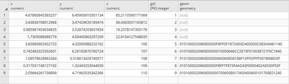
After applying the general update, then all the registers will have a value on their geom column:
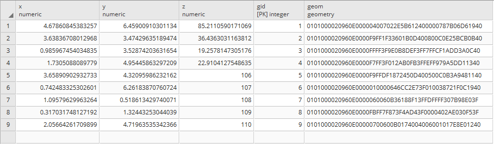
So far, we've implemented an insert trigger. What if the value changes for a particular row? In that case, we will require a separate update trigger. We'll change our original function to test the UPDATE case, and we'll use WHEN in our trigger to constrain updates to the column being changed.
Also, note that the following function is written with the assumption that the user wants to always update the changing geometries based on the changing values:
CREATE OR REPLACE FUNCTION chp02.before_insertXYZ()
  RETURNS trigger AS
$$
BEGIN
if (TG_OP='INSERT') then
  if (NEW.geom is null) then
    NEW.geom = ST_SetSRID(ST_MakePoint(NEW.x,NEW.y), 3734);
  end if;
ELSEIF (TG_OP='UPDATE') then
  NEW.geom = ST_SetSRID(ST_MakePoint(NEW.x,NEW.y), 3734);
end if;
RETURN NEW;
END;

$$
LANGUAGE 'plpgsql';

CREATE TRIGGER popgeom_insert
  BEFORE INSERT ON chp02.xwhyzed1
  FOR EACH ROW EXECUTE PROCEDURE chp02.before_insertXYZ();

CREATE trigger popgeom_update
  BEFORE UPDATE ON chp02.xwhyzed1
  FOR EACH ROW
  WHEN (OLD.X IS DISTINCT FROM NEW.X OR OLD.Y IS DISTINCT FROM
    NEW.Y)
  EXECUTE PROCEDURE chp02.before_insertXYZ();
An unusual and useful property of the PostgreSQL database is that it allows for object inheritance models as they apply to tables. This means that we can have parent/child relationships between tables and leverage that to structure the data in meaningful ways. In our example, we will apply this to hydrology data. This data can be points, lines, polygons, or more complex structures, but they have one commonality: they are explicitly linked in a physical sense and inherently related; they are all about water. Water/hydrology is an excellent natural system to model this way, as our ways of modeling it spatially can be quite mixed depending on scales, details, the data collection process, and a host of other factors.
The data we will be using is hydrology data that has been modified from engineering blue lines (see the following screenshot), that is, hydrologic data that is very detailed and is meant to be used at scales approaching 1:600. The data in its original application aided, as breaklines, in detailed digital terrain modeling.
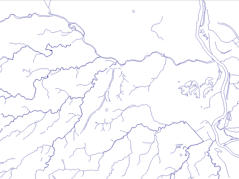
While useful in itself, the data was further manipulated, separating the linear features from area features, with additional polygonization of the area features, as shown in the following screenshot:
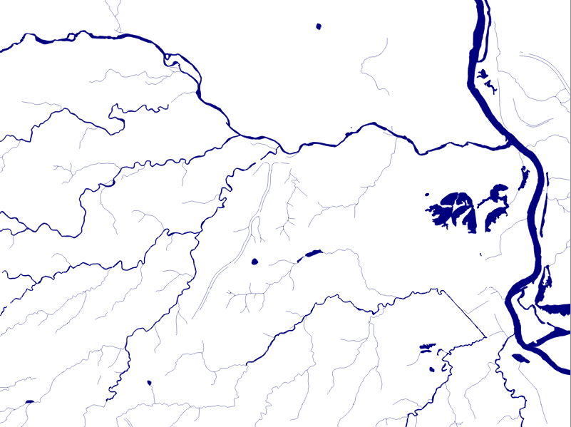
Finally, the data was classified into basic waterway categories, as follows:
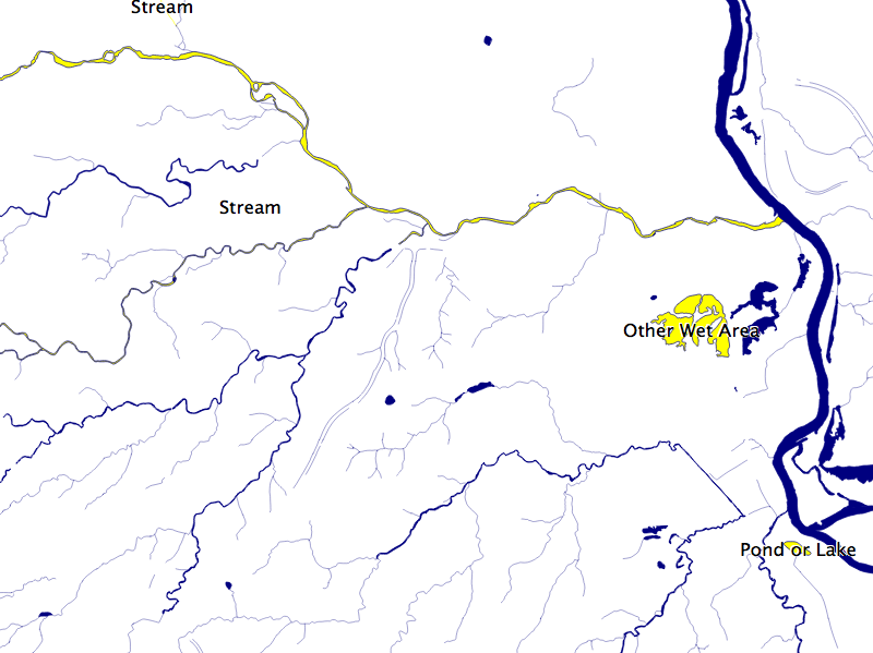
In addition, a process was undertaken to generate centerlines for polygon features such as streams, which are effectively linear features, as follows:
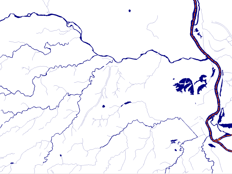
Hence, we have three separate but related datasets:
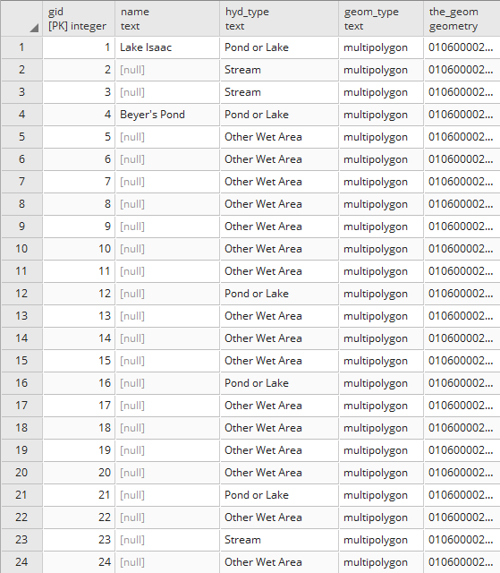
Now, let us look at the structure of the tabular data. Unzip the hydrology file from the book repository and go to that directory. The ogrinfo utility can help us with this, as shown in the following command:
> ogrinfo cuyahoga_hydro_polygon.shp -al -so
The output is as follows:
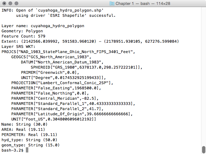
Executing this query on each of the shapefiles, we see the following fields that are common to all the shapefiles:
It is by understanding our common fields that we can apply inheritance to completely structure our data.
Now that we know our common fields, creating an inheritance model is easy. First, we will create a parent table with the fields common to all the tables, using the following query:
CREATE TABLE chp02.hydrology (
  gid SERIAL PRIMARY KEY,
  "name"      text,
  hyd_type    text,
  geom_type   text,
  the_geom    geometry
);
If you are paying attention, you will note that we also added a geometry field as all of our shapefiles implicitly have this commonality. With inheritance, every record inserted in any of the child tables will also be saved in our parent table, only these records will be stored without the extra fields specified for the child tables.
To establish inheritance for a given table, we need to declare only the additional fields that the child table contains using the following query:
CREATE TABLE chp02.hydrology_centerlines (
  "length"    numeric
) INHERITS (chp02.hydrology);

CREATE TABLE chp02.hydrology_polygon (
  area    numeric,
  perimeter    numeric
) INHERITS (chp02.hydrology);

CREATE TABLE chp02.hydrology_linestring (
  sinuosity    numeric
) INHERITS (chp02.hydrology_centerlines);
Now, we are ready to load our data using the following commands:
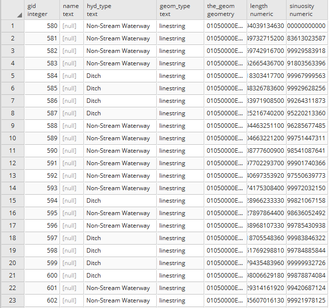
If we view our parent table, we will see all the records in all the child tables. The following is a screenshot of fields in hydrology:
Compare that to the fields available in hydrology_linestring that will reveal specific fields of interest:
PostgreSQL table inheritance allows us to enforce essentially hierarchical relationships between tables. In this case, we leverage inheritance to allow for commonality between related datasets. Now, if we want to query data from these tables, we can query directly from the parent table as follows, depending on whether we want a mix of geometries or just a targeted dataset:
SELECT * FROM chp02.hydrology
From any of the child tables, we could use the following query:
SELECT * FROM chp02.hydrology_polygon
It is possible to extend this concept in order to leverage and optimize storage and querying by using the CHECK constrains in conjunction with inheritance. For more info, see the Extending inheritance – table partitioning recipe.
Table partitioning is an approach specific to PostgreSQL that extends inheritance to model tables that typically do not vary from each other in the available fields, but where the child tables represent logical partitioning of the data based on a variety of factors, be it time, value ranges, classifications, or in our case, spatial relationships. The advantages of partitioning include improved query performance due to smaller indexes and targeted scans of data, bulk loads, and deletes that bypass the costs of vacuuming. It can thus be used to put commonly used data on faster and more expensive storage, and the remaining data on slower and cheaper storage. In combination with PostGIS, we get the novel power of spatial partitioning, which is a really powerful feature for large datasets.
We could use many examples of large datasets that could benefit from partitioning. In our case, we will use a contour dataset. Contours are useful ways to represent terrain data, as they are well established and thus commonly interpreted. Contours can also be used to compress terrain data into linear representations, thus allowing it to be shown in conjunction with other data easily.
The problem is, the storage of contour data can be quite expensive. Two-foot contours for a single US county can take 20 to 40 GB, and storing such data for a larger area such as a region or nation can become quite prohibitive from the standpoint of accessing the appropriate portion of the dataset in a performant way.
The first step in this case may be to prepare the data. If we had a monolithic contour table called cuy_contours_2, we could choose to clip the data to a series of rectangles that will serve as our table partitions; in this case, chp02.contour_clip, using the following query:
CREATE TABLE chp02.contour_2_cm_only AS
  SELECT contour.elevation, contour.gid, contour.div_10, contour.div_20, contour.div_50,
  contour.div_100, cc.id, ST_Intersection(contour.the_geom, cc.the_geom) AS the_geom FROM
    chp02.cuy_contours_2 AS contour, chp02.contour_clip as cc
    WHERE ST_Within(contour.the_geom,cc.the_geom
      OR
      ST_Crosses(contour.the_geom,cc.the_geom);
We are performing two tests here in our query. We are using ST_Within, which tests whether a given contour is entirely within our area of interest. If so, we perform an intersection; the resultant geometry should just be the geometry of the contour.
The ST_Crosses function checks whether the contour crosses the boundary of the geometry we are testing. This should capture all the geometries lying partially inside and partially outside our areas. These are the ones that we will truly intersect to get the resultant shape.
In our case, it is easier and we don't require this step. Our contour shapes are already individual shapefiles clipped to rectangular boundaries, as shown in the following screenshot:
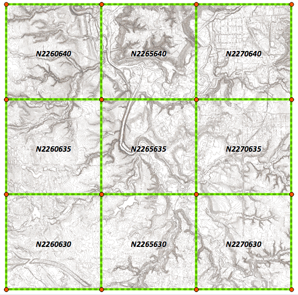
Since the data is already clipped into the chunks needed for our partitions, we can just continue to create the appropriate partitions.
Much like with inheritance, we start by creating our parent table using the following query:
CREATE TABLE chp02.contours
(
  gid serial NOT NULL,
  elevation integer,
  __gid double precision,
  the_geom geometry(MultiLineStringZM,3734),
  CONSTRAINT contours_pkey PRIMARY KEY (gid)
)
WITH (
  OIDS=FALSE
);
Here again, we maintain our constraints, such as PRIMARY KEY, and specify the geometry type (MultiLineStringZM), not because these will propagate to the child tables, but for any client software accessing the parent table to anticipate such constraints.
Now we may begin to create tables that inherit from our parent table. In the process, we will create a CHECK constraint specifying the limits of our associated geometry using the following query:
CREATE TABLE chp02.contour_N2260630
  (CHECK
    (ST_CoveredBy(the_geom,ST_GeomFromText
      ('POLYGON((2260000, 630000, 2260000 635000, 2265000 635000,
                 2265000 630000, 2260000 630000))',3734)
    )
  )) INHERITS (chp02.contours);
We can complete the table structure for partitioning the contours with similar CREATE TABLE queries for our remaining tables, as follows:
CREATE TABLE chp02.contour_N2260635
  (CHECK
    (ST_CoveredBy(the_geom,ST_GeomFromText
      ('POLYGON((2260000 635000, 2260000 640000,
                 2265000 640000, 2265000 635000, 2260000 635000))', 3734)
    )
  )) INHERITS (chp02.contours);
CREATE TABLE chp02.contour_N2260640
  (CHECK
    (ST_CoveredBy(the_geom,ST_GeomFromText
      ('POLYGON((2260000 640000, 2260000 645000, 2265000 645000,
                 2265000 640000, 2260000 640000))', 3734)
    )
  )) INHERITS (chp02.contours);
CREATE TABLE chp02.contour_N2265630
  (CHECK
    (ST_CoveredBy(the_geom,ST_GeomFromText
      ('POLYGON((2265000 630000, 2265000 635000, 2270000 635000,
                 2270000 630000, 2265000 630000))', 3734)
    )
  )) INHERITS (chp02.contours);
CREATE TABLE chp02.contour_N2265635
  (CHECK
    (ST_CoveredBy(the_geom,ST_GeomFromText
      ('POLYGON((2265000 635000, 2265000 640000, 2270000 640000,
                 2270000 635000, 2265000 635000))', 3734)
    )
  )) INHERITS (chp02.contours);
CREATE TABLE chp02.contour_N2265640
  (CHECK
    (ST_CoveredBy(the_geom,ST_GeomFromText
      ('POLYGON((2265000 640000, 2265000 645000, 2270000 645000,
                 2270000 640000, 2265000 640000))', 3734)
    )
  )) INHERITS (chp02.contours);
CREATE TABLE chp02.contour_N2270630
  (CHECK
    (ST_CoveredBy(the_geom,ST_GeomFromText
      ('POLYGON((2270000 630000, 2270000 635000, 2275000 635000,
                 2275000 630000, 2270000 630000))', 3734)
    )
  )) INHERITS (chp02.contours);
CREATE TABLE chp02.contour_N2270635
  (CHECK
    (ST_CoveredBy(the_geom,ST_GeomFromText
      ('POLYGON((2270000 635000, 2270000 640000, 2275000 640000,
                 2275000 635000, 2270000 635000))', 3734)
    )
  )) INHERITS (chp02.contours);
CREATE TABLE chp02.contour_N2270640
  (CHECK
    (ST_CoveredBy(the_geom,ST_GeomFromText
      ('POLYGON((2270000 640000, 2270000 645000, 2275000 645000,
                 2275000 640000, 2270000 640000))', 3734)
    )
  )) INHERITS (chp02.contours);
And now we can load our contours shapefiles found in the contours1 ZIP file into each of our child tables, using the following command, by replacing the filename. If we wanted to, we could even implement a trigger on the parent table, which would place each insert into its correct child table, though this might incur performance costs:
shp2pgsql -s 3734 -a -i -I -W LATIN1 -g the_geom N2265630 chp02.contour_N2265630 | psql -U me -d postgis_cookbook
The CHECK constraint in combination with inheritance is all it takes to build a table partitioning. In this case, we're using a bounding box as our CHECK constraint and simply inheriting the columns from the parent table. Now that we have this in place, queries against the parent table will check our CHECK constraints first before employing a query.
This also allows us to place any of our lesser-used contour tables on cheaper and slower storage, thus allowing for cost-effective optimizations of large datasets. This structure is also beneficial for rapidly changing data, as updates can be applied to an entire area; the entire table for that area can be efficiently dropped and repopulated without traversing across the dataset.
For more on table inheritance in general, particularly the flexibility associated with the usage of alternate columns in the child table, see the previous recipe, Structuring spatial data with table inheritance.
Often, data used in a spatial database is imported from other sources. As such, it may not be in a form that is useful for our current application. In such a case, it may be useful to write functions that will aid in transforming the data into a form that is more useful for our application. This is particularly the case when going from flat file formats, such as shapefiles, to relational databases such as PostgreSQL.
There are many structures that might serve as a proxy for relational stores in a shapefile. We will explore one here: a single field with delimited text for multiple relations. This is a not-too-uncommon hack to encode multiple relationships into a flat file. The other common approach is to create multiple fields to store what in a relational arrangement would be a single field.
The dataset we will be working with is a trails dataset that has linear extents for a set of trails in a park system. The data is the typical data that comes from the GIS world; as a flat shapefile, there are no explicit relational constructs in the data.
First, unzip the trails.zip file and use the command line to go into it, then load the data using the following command:
shp2pgsql -s 3734 -d -i -I -W LATIN1 -g the_geom trails chp02.trails | psql -U me -d postgis_cookbook
Looking at the linear data, we have some categories for the use type:
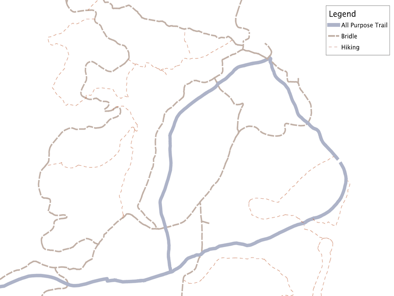
We want to retain this information as well as the name. Unfortunately, the label_name field is a messy field with a variety of related names concatenated with an ampersand (&), as shown in the following query:
SELECT DISTINCT label_name FROM chp02.trails
  WHERE label_name LIKE '%&%' LIMIT 10;
It will return the following output:
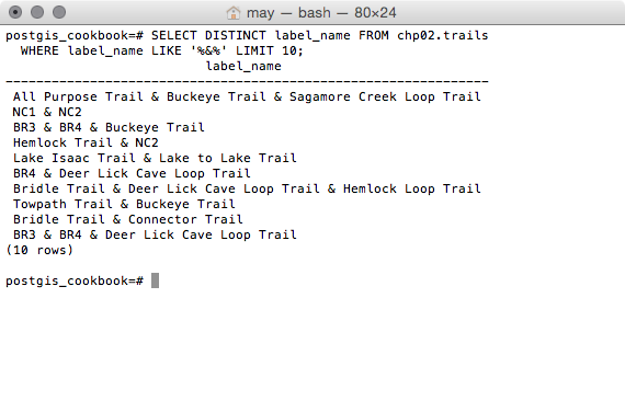
This is where the normalization of our table will begin.
The first thing we need to do is find all the fields that don't have ampersands and use those as our unique list of available trails. In our case, we can do this, as every trail has at least one segment that is uniquely named and not associated with another trail name. This approach will not work with all datasets, so be careful in understanding your data before applying this approach to that data.
To select the fields ordered without ampersands, we use the following query:
SELECT DISTINCT label_name, res
  FROM chp02.trails
  WHERE label_name NOT LIKE '%&%'
  ORDER BY label_name, res;
It will return the following output:
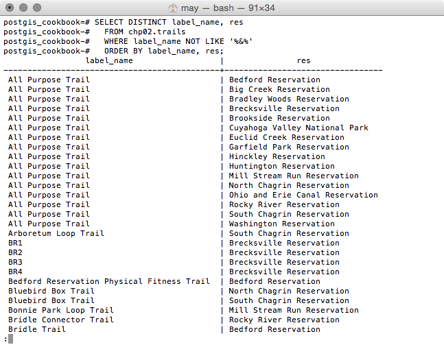
Next, we want to search for all the records that match any of these unique trail names. This will give us the list of records that will serve as relations. The first step in doing this search is to append the percent (%) signs to our unique list in order to build a string on which we can search using a LIKE query:
SELECT '%' || label_name || '%' AS label_name, label_name as   label, res FROM
  (SELECT DISTINCT label_name, res
    FROM chp02.trails
    WHERE label_name NOT LIKE '%&%'
    ORDER BY label_name, res
  ) AS label;
Finally, we'll use this in the context of a WITH block to do the normalization itself. This will provide us with a table of unique IDs for each segment in our first column, along with the associated label column. For good measure, we will do this as a CREATE TABLE procedure, as shown in the following query:
CREATE TABLE chp02.trails_names AS WITH labellike AS
(
SELECT '%' || label_name || '%' AS label_name, label_name as   label, res FROM
  (SELECT DISTINCT label_name, res
    FROM chp02.trails
    WHERE label_name NOT LIKE '%&%'
    ORDER BY label_name, res
  ) AS label
)
SELECT t.gid, ll.label, ll.res
  FROM chp02.trails AS t, labellike AS ll
  WHERE t.label_name LIKE ll.label_name
  AND
  t.res = ll.res
  ORDER BY gid;
If we view the first rows of the table created, trails_names, we have the following output with pgAdmin:
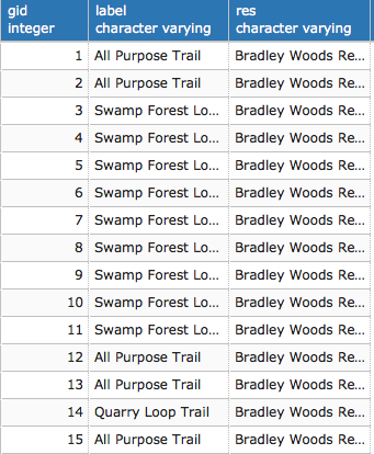
Now that we have a table of the relations, we need a table of the geometries associated with gid. This, in comparison, is quite easy, as shown in the following query:
CREATE TABLE chp02.trails_geom AS
  SELECT gid, the_geom
  FROM chp02.trails;
In this example, we have generated a unique list of possible records in conjunction with a search for the associated records, in order to build table relationships. In one table, we have the geometry and a unique ID of each spatial record; in another table, we have the names associated with each of those unique IDs. Now we can explicitly leverage those relationships.
First, we need to establish our unique IDs as primary keys, as follows:
ALTER TABLE chp02.trails_geom ADD PRIMARY KEY (gid);
Now we can use that PRIMARY KEY as a FOREIGN KEY in our trails_names table using the following query:
ALTER TABLE chp02.trails_names ADD FOREIGN KEY (gid) REFERENCES chp02.trails_geom(gid);
This step isn't strictly necessary, but does enforce referential integrity for queries such as the following:
SELECT geo.gid, geo.the_geom, names.label FROM
  chp02.trails_geom AS geo, chp02.trails_names AS names
  WHERE geo.gid = names.gid;
The output is as follows:
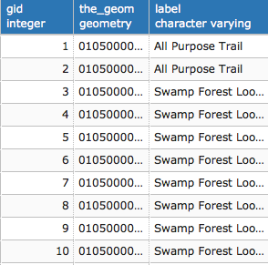
If we had multiple fields we wanted to normalize, we could write CREATE TABLE queries for each of them.
It is interesting to note that the approach framed in this recipe is not limited to cases where we have a delimited field. This approach can provide a relatively generic solution to the problem of normalizing flat files. For example, if we have a case where we have multiple fields to represent relational info, such as label1, label2, label3, or similar multiple attribute names for a single record, we can write a simple query to concatenate them together before feeding that info into our query.
Data from an external source can have issues in the table structure as well as in the topology, endemic to the geospatial data itself. Take, for example, the problem of data with overlapping polygons. If our dataset has polygons that overlap with internal overlays, then queries for area, perimeter, and other metrics may not produce predictable or consistent results.
There are a few approaches that can solve the problem of polygon datasets with internal overlays. The general approach presented here was originally proposed by Kevin Neufeld of Refractions Research.
Over the course of writing our query, we will also produce a solution for converting polygons to linestrings.
First, unzip the use_area.zip file and go into it using the command line; then, load the dataset using the following command:
shp2pgsql -s 3734 -d -i -I -W LATIN1 -g the_geom cm_usearea_polygon chp02.use_area | psql -U me -d postgis_cookbook
Now that the data is loaded into a table in the database, we can leverage PostGIS to flatten and get the union of the polygons, so that we have a normalized dataset. The first step in doing so using this approach will be to convert the polygons to linestrings. We can then link those linestrings and convert them back to polygons, representing the union of all the polygon inputs. We will perform the following tasks:
To convert polygons to linestrings, we'll need to extract just the portions of the polygons we want using ST_ExteriorRing, convert those parts to points using ST_DumpPoints, and then connect those points back into lines like a connect-the-dots coloring book using ST_MakeLine.
Breaking it down further, ST_ExteriorRing (the_geom) will grab just the outer boundary of our polygons. But ST_ExteriorRing returns polygons, so we need to take that output and create a line from it. The easiest way to do this is to convert it to points using ST_DumpPoints and then connect those points. By default, the Dump function returns an object called a geometry_dump, which is not just simple geometry, but the geometry in combination with an array of integers. The easiest way to return the geometry alone is the leverage object notation to extract just the geometry portion of geometry_dump, as follows:
(ST_DumpPoints(geom)).geom
Piecing the geometry back together with ST_ExteriorRing is done using the following query:
SELECT (ST_DumpPoints(ST_ExteriorRing(geom))).geom
This should give us a listing of points in order from the exterior rings of all the points from which we want to construct our lines using ST_MakeLine, as shown in the following query:
SELECT ST_MakeLine(geom) FROM (
  SELECT (ST_DumpPoints(ST_ExteriorRing(geom))).geom) AS linpoints
Since the preceding approach is a process we may want to use in many other places, it might be prudent to create a function from this using the following query:
CREATE OR REPLACE FUNCTION chp02.polygon_to_line(geometry)
  RETURNS geometry AS
$BODY$

  SELECT ST_MakeLine(geom) FROM (
    SELECT (ST_DumpPoints(ST_ExteriorRing((ST_Dump($1)).geom))).geom

  ) AS linpoints
$BODY$
  LANGUAGE sql VOLATILE;
ALTER FUNCTION chp02.polygon_to_line(geometry)
  OWNER TO me;
Now that we have the polygon_to_line function, we still need to force the linking of overlapping lines in our particular case. The ST_Union function will aid in this, as shown in the following query:
SELECT ST_Union(the_geom) AS geom FROM (
  SELECT chp02.polygon_to_line(geom) AS geom FROM
    chp02.use_area
  ) AS unioned;
Now let's convert linestrings back to polygons, and for this we can polygonize the result using ST_Polygonize, as shown in the following query:
SELECT ST_Polygonize(geom) AS geom FROM (
  SELECT ST_Union(the_geom) AS geom FROM (
    SELECT chp02.polygon_to_line(geom) AS geom FROM
    chp02.use_area
  ) AS unioned
) as polygonized;
The ST_Polygonize function will create a single multi polygon, so we need to explode this into multiple single polygon geometries if we are to do anything useful with it. While we are at it, we might as well do the following within a CREATE TABLE statement:
CREATE TABLE chp02.use_area_alt AS (
  SELECT (ST_Dump(the_geom)).geom AS the_geom FROM (
    SELECT ST_Polygonize(the_geom) AS the_geom FROM (
      SELECT ST_Union(the_geom) AS the_geom FROM (
        SELECT chp02.polygon_to_line(the_geom) AS the_geom
        FROM chp02.use_area
      ) AS unioned
    ) as polygonized
  ) AS exploded
);
We will be performing spatial queries against this geometry, so we should create an index in order to ensure our query performs well, as shown in the following query:
CREATE INDEX chp02_use_area_alt_the_geom_gist
  ON chp02.use_area_alt
  USING gist(the_geom);
In order to find the appropriate table information from the original geometry and apply that back to our resultant geometries, we will perform a point-in-polygon query. For that, we first need to calculate centroids on the resultant geometry:
CREATE TABLE chp02.use_area_alt_p AS
  SELECT ST_SetSRID(ST_PointOnSurface(the_geom), 3734) AS
    the_geom FROM
    chp02.use_area_alt;
ALTER TABLE chp02.use_area_alt_p ADD COLUMN gid serial;
ALTER TABLE chp02.use_area_alt_p ADD PRIMARY KEY (gid);
And as always, create a spatial index using the following query:
CREATE INDEX chp02_use_area_alt_p_the_geom_gist
  ON chp02.use_area_alt_p
  USING gist(the_geom);
The centroids then structure our point-in-polygon (ST_Intersects) relationship between the original tabular information and resultant polygons, using the following query:
CREATE TABLE chp02.use_area_alt_relation AS
SELECT points.gid, cu.location FROM
  chp02.use_area_alt_p AS points,
  chp02.use_area AS cu
    WHERE ST_Intersects(points.the_geom, cu.the_geom);
If we view the first rows of the table, we can see it links the identifier of points to their respective locations:
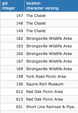
Our essential approach here is to look at the underlying topology of the geometry and reconstruct a topology that is non-overlapping, and then use the centroids of that new geometry to construct a query that establishes the relationship to the original data.
At this stage, we can optionally establish a framework for referential integrity using a foreign key, as follows:
ALTER TABLE chp02.use_area_alt_relation ADD FOREIGN KEY (gid) REFERENCES chp02.use_area_alt_p (gid);
PostgreSQL functions abound for the aggregation of tabular data, including sum, count, min, max, and so on. PostGIS as a framework does not explicitly have spatial equivalents of these, but this does not prevent us from building functions using the aggregate functions from PostgreSQL in concert with PostGIS's spatial functionality.
In this recipe, we will explore spatial summarization with the United States census data. The US census data, by nature, is aggregated data. This is done intentionally to protect the privacy of citizens. But when it comes to doing analyses with this data, the aggregate nature of the data can become problematic. There are some tricks to disaggregate data. Amongst the simplest of these is the use of a proportional sum, which we will do in this exercise.
The problem at hand is that a proposed trail has been drawn in order to provide services for the public. This example could apply to road construction or even finding sites for commercial properties for the purpose of provisioning services.
First, unzip the trail_census.zip file, then perform a quick data load using the following commands from the unzipped folder:
shp2pgsql -s 3734 -d -i -I -W LATIN1 -g the_geom census chp02.trail_census | psql -U me -d postgis_cookbook
shp2pgsql -s 3734 -d -i -I -W LATIN1 -g the_geom trail_alignment_proposed_buffer chp02.trail_buffer | psql -U me -d postgis_cookbook
shp2pgsql -s 3734 -d -i -I -W LATIN1 -g the_geom trail_alignment_proposed chp02.trail_alignment_prop | psql -U me -d postgis_cookbook
The preceding commands will produce the following outputs:
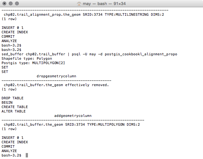
If we view the proposed trail in our favorite desktop GIS, we have the following:
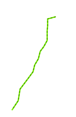
In our case, we want to know the population within 1 mile of the trail, assuming that persons living within 1 mile of the trail are the ones most likely to use it, and thus most likely to be served by it.
To find out the population near this proposed trail, we overlay census block group population density information. Illustrated in the next screenshot is a 1-mile buffer around the proposed trail:
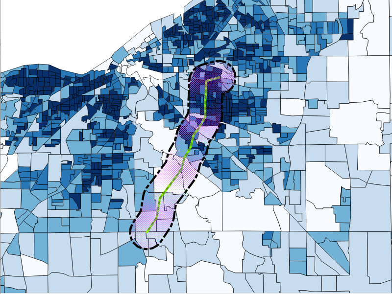
One of the things we might note about this census data is the wide range of census densities and census block group sizes. An approach to calculating the population would be to simply select all census blocks that intersect our area, as shown in the following screenshot:
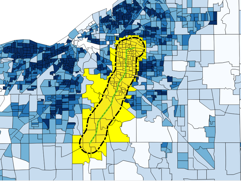
This is a simple procedure that gives us an estimate of 130 to 288 people living within 1 mile of the trail, but looking at the shape of the selection, we can see that we are overestimating the population by taking the complete blocks in our estimate.
Similarly, if we just used the block groups whose centroids lay within 1 mile of our proposed trail alignment, we would underestimate the population.
Instead, we will make some useful assumptions. Block groups are designed to be moderately homogeneous within the block group population distribution. Assuming that this holds true for our data, we can assume that for a given block group, if 50% of the block group is within our target area, we can attribute half of the population of that block group to our estimate. Apply this to all our block groups, sum them, and we have a refined estimate that is likely to be better than pure intersects or centroid queries. Thus, we employ a proportional sum.
As the problem of a proportional sum is a generic problem, it could apply to many problems. We will write the underlying proportioning as a function. A function takes inputs and returns a value. In our case, we want our proportioning function to take two geometries, that is, the geometry of our buffered trail and block groups as well as the value we want proportioned, and we want it to return the proportioned value:
CREATE OR REPLACE FUNCTION chp02.proportional_sum(geometry,   geometry, numeric)
  RETURNS numeric AS
$BODY$
-- SQL here
$BODY$
  LANGUAGE sql VOLATILE;
Now, for the purpose of our calculation, for any given intersection of buffered area and block group, we want to find the proportion that the intersection is over the overall block group. Then this value should be multiplied by the value we want to scale.
In SQL, the function looks like the following query:
SELECT $3 * areacalc FROM
  (SELECT (ST_Area(ST_Intersection($1, $2)) / ST_Area($2)):: numeric AS areacalc
  ) AS areac;
The preceding query in its full form looks as follows:
CREATE OR REPLACE FUNCTION chp02.proportional_sum(geometry,   geometry, numeric)
  RETURNS numeric AS
$BODY$
    SELECT $3 * areacalc FROM
      (SELECT (ST_Area(ST_Intersection($1,           $2))/ST_Area($2))::numeric AS areacalc
      ) AS areac
;
$BODY$
  LANGUAGE sql VOLATILE;
Since we have written the query as a function, the query uses the SELECT statement to loop through all available records and give us a proportioned population. Astute readers will note that we have not yet done any work on summarization; we have only worked on the proportionality portion of the problem. We can do the summarization upon calling the function using PostgreSQL's built-in aggregate functions. What is neat about this approach is that we need not just apply a sum, but we could also calculate other aggregates such as min or max. In the following example, we will just apply a sum:
SELECT ROUND(SUM(chp02.proportional_sum(a.the_geom, b.the_geom, b.pop))) FROM
  chp02.trail_buffer AS a, chp02.trail_census as b
  WHERE ST_Intersects(a.the_geom, b.the_geom)
  GROUP BY a.gid;
The value returned is quite different (a population of 96,081), which is more likely to be accurate.
In this chapter, we will cover the following recipes:
In this chapter, you will work with a set of PostGIS functions and vector datasets. You will first take a look at how to use PostGIS with GPS data—you will import such datasets using ogr2ogr and then compose polylines from point geometries using the ST_MakeLine function.
Then, you will see how PostGIS helps you find and fix invalid geometries with functions such as ST_MakeValid, ST_IsValid, ST_IsValidReason, and ST_IsValidDetails.
You will then learn about one of the most powerful elements of a spatial database, spatial joins. PostGIS provides you with a rich set of operators, such as ST_Intersects, ST_Contains, ST_Covers, ST_Crosses, and ST_DWithin, for this purpose.
After that, you will use the ST_Simplify and ST_SimplifyPreverveTopology functions to simplify (generalize) geometries when you don't need too many details. While this function works well on linear geometries, topological anomalies may be introduced for polygonal ones. In such cases, you should consider using an external GIS tool such as GRASS.
You will then have a tour of PostGIS functions to make distance measurements—ST_Distance, ST_DistanceSphere, and ST_DistanceSpheroid are on the way.
One of the recipes explained in this chapter will guide you through the typical GIS workflow to merge polygons based on a common attribute; you will use the ST_Union function for this purpose.
You will then learn how to clip geometries using the ST_Intersection function, before deep diving into the PostGIS topology in the last recipe that was introduced in version 2.0.
In this recipe, you will work with GPS data. This kind of data is typically saved in a .gpx file. You will import a bunch of .gpx files to PostGIS from RunKeeper, a popular social network for runners.
If you have an account on RunKeeper, you can export your .gpx files and process them by following the instructions in this recipe. Otherwise, you can use the RunKeeper .gpx files included in the runkeeper-gpx.zip file located in the chp03 directory available in the code bundle for this book.
You will first create a bash script for importing the .gpx files to a PostGIS table, using ogr2ogr. After the import is completed, you will try to write a couple of SQL queries and test some very useful functions, such as ST_MakeLine to generate polylines from point geometries, ST_Length to compute distance, and ST_Intersects to perform a spatial join operation.
Extract the data/chp03/runkeeper-gpx.zip file to working/chp03/runkeeper_gpx. In case you haven't been through Chapter 1, Moving Data In and Out of PostGIS, be sure to have the countries dataset in the PostGIS database.
First, be sure of the format of the .gpx files that you need to import to PostGIS. Open one of them and check the file structure—each file must be in the XML format composed of just one <trk> element, which contains just one <trkseg> element, which contains many <trkpt> elements (the points stored from the runner's GPS device). Import these points to a PostGIS Point table:
postgis_cookbook=# create schema chp03;
      postgis_cookbook=# CREATE TABLE chp03.rk_track_points
      (
        fid serial NOT NULL,
        the_geom geometry(Point,4326),
        ele double precision,
        "time" timestamp with time zone,
        CONSTRAINT activities_pk PRIMARY KEY (fid)
      );
The following is the Linux version (name it working/chp03/import_gpx.sh):
        #!/bin/bash
        for f in `find runkeeper_gpx -name \*.gpx -printf "%f\n"`
        do
          echo "Importing gpx file $f to chp03.rk_track_points
                PostGIS table..." #, ${f%.*}"
          ogr2ogr -append -update  -f PostgreSQL
          PG:"dbname='postgis_cookbook' user='me'
          password='mypassword'" runkeeper_gpx/$f
          -nln chp03.rk_track_points
          -sql "SELECT ele, time FROM track_points"
        done
The following is the command for macOS (name it working/chp03/import_gpx.sh):
        #!/bin/bash
        for f in `find runkeeper_gpx -name \*.gpx `
        do
          echo "Importing gpx file $f to chp03.rk_track_points
                PostGIS table..." #, ${f%.*}"
          ogr2ogr -append -update  -f PostgreSQL
          PG:"dbname='postgis_cookbook' user='me'
          password='mypassword'" $f
          -nln chp03.rk_track_points
          -sql "SELECT ele, time FROM track_points"
        done
The following is the Windows version (name it working/chp03/import_gpx.bat):
        @echo off
        for %%I in (runkeeper_gpx\*.gpx*) do (
          echo Importing gpx file %%~nxI to chp03.rk_track_points
               PostGIS table...
          ogr2ogr -append -update -f PostgreSQL
          PG:"dbname='postgis_cookbook' user='me'
          password='mypassword'" runkeeper_gpx/%%~nxI
          -nln chp03.rk_track_points
          -sql "SELECT ele, time FROM track_points"
        )
      $ chmod 775 import_gpx.sh
      $ ./import_gpx.sh
      Importing gpx file 2012-02-26-0930.gpx to chp03.rk_track_points
        PostGIS table...
      Importing gpx file 2012-02-29-1235.gpx to chp03.rk_track_points
        PostGIS table...
      ...
      Importing gpx file 2011-04-15-1906.gpx to chp03.rk_track_points
        PostGIS table...
In Windows, just double-click on the .bat file or run it from the command prompt using the following command:
> import_gpx.bat
      postgis_cookbook=# SELECT
      ST_MakeLine(the_geom) AS the_geom,
      run_date::date,
      MIN(run_time) as start_time,
      MAX(run_time) as end_time
      INTO chp03.tracks
      FROM (
        SELECT the_geom,
        "time"::date as run_date,
        "time" as run_time
        FROM chp03.rk_track_points
        ORDER BY run_time
      ) AS foo GROUP BY run_date;
      postgis_cookbook=# CREATE INDEX rk_track_points_geom_idx
      ON chp03.rk_track_points USING gist(the_geom);
      postgis_cookbook=# CREATE INDEX tracks_geom_idx
      ON chp03.tracks USING gist(the_geom);
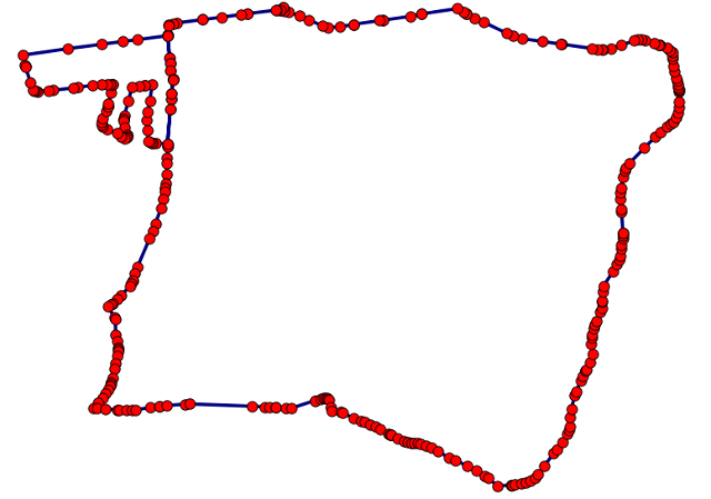
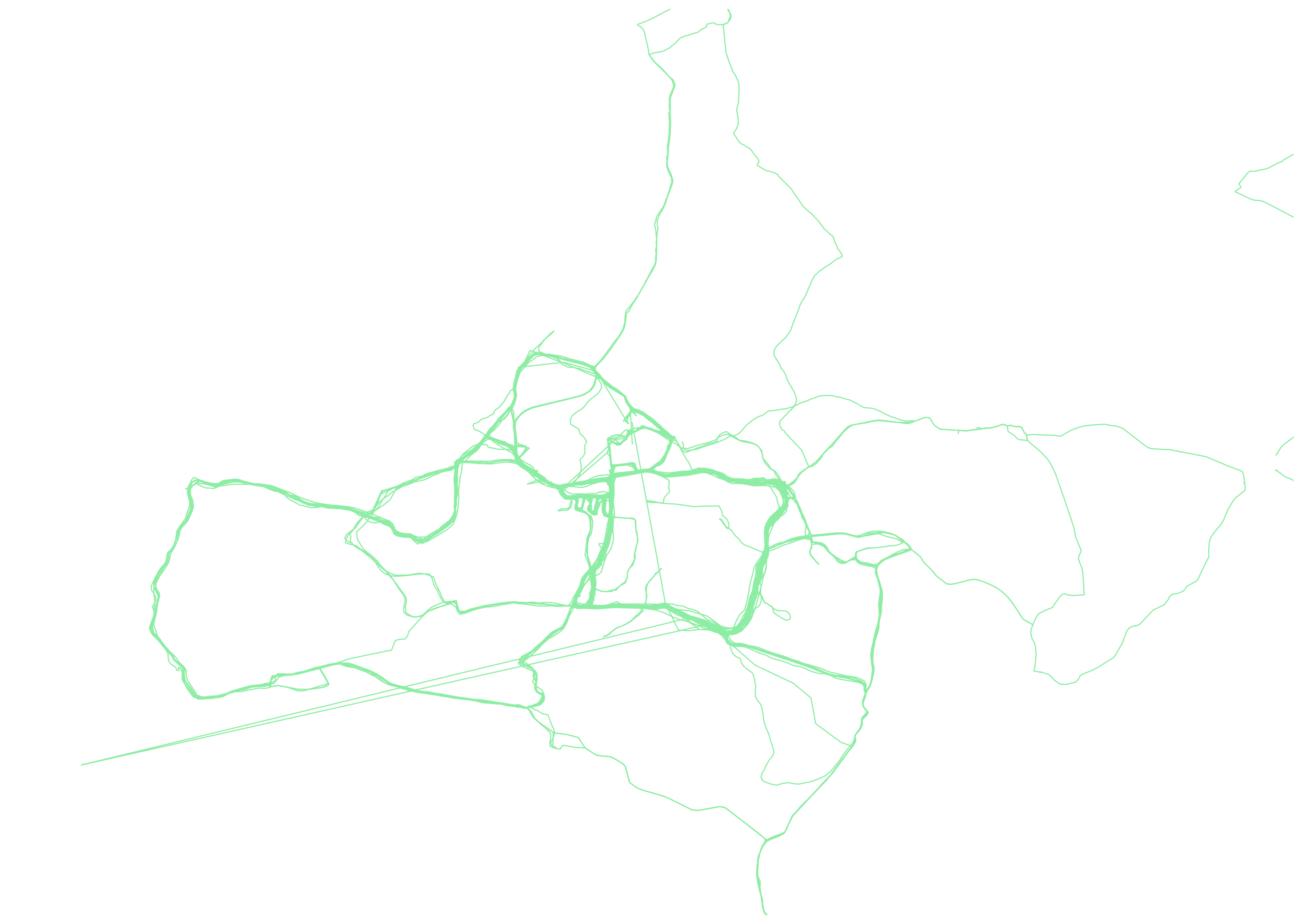
      postgis_cookbook=# SELECT
        EXTRACT(year FROM run_date) AS run_year,
        EXTRACT(MONTH FROM run_date) as run_month,
        SUM(ST_Length(geography(the_geom)))/1000 AS distance
        FROM chp03.tracks
        GROUP BY run_year, run_month ORDER BY run_year, run_month;
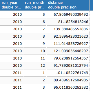
(28 rows)
      postgis_cookbook=# SELECT
        c.country_name,
        SUM(ST_Length(geography(t.the_geom)))/1000 AS run_distance
      FROM chp03.tracks AS t
      JOIN chp01.countries AS c
      ON ST_Intersects(t.the_geom, c.the_geom)
      GROUP BY c.country_name
      ORDER BY run_distance DESC;
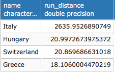
(4 rows)
The .gpx files store all the points' details in the WGS 84 spatial reference system; therefore, we created the rk_track_points table with SRID (4326).
After creating the rk_track_points table, we imported all of the .gpx files in the runkeeper_gpx directory using a bash script. The bash script iterates all of the files with the extension *.gpx in the runkeeper_gpx directory. For each of these files, the script runs the ogr2ogr command, importing the .gpx files to PostGIS using the GPX GDAL driver (for more details, go to http://www.gdal.org/drv_gpx.html).
In the GDAL's abstraction, a .gpx file is an OGR data source composed of several layers as follows:
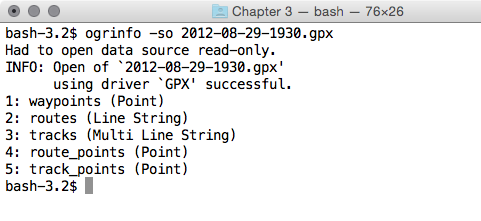
In the .gpx files (OGR data sources), you have just the tracks and track_points layers. As a shortcut, you could have imported just the tracks layer using ogr2ogr, but you would need to start from the track_points layer in order to generate the tracks layer itself, using some PostGIS functions. This is why in the ogr2ogr section in the bash script, we imported to the rk_track_points PostGIS table the point geometries from the track_points layer, plus a couple of useful attributes, such as elevation and timestamp.
Once the records were imported, we fed a new polylines table named tracks using a subquery and selected all of the point geometries and their dates and times from the rk_track_points table, grouped by date and with the geometries aggregated using the ST_MakeLine function. This function was able to create linestrings from point geometries (for more details, go to http://www.postgis.org/docs/ST_MakeLine.html).
You should not forget to sort the points in the subquery by datetime; otherwise, you will obtain an irregular linestring, jumping from one point to the other and not following the correct order.
After loading the tracks table, we tested the two spatial queries.
At first, you got a month-by-month report of the total distance run by the runner. For this purpose, you selected all of the track records grouped by date (year and month), with the total distance obtained by summing up the lengths of the single tracks (obtained with the ST_Length function). To get the year and the month from the run_date function, you used the PostgreSQL EXTRACT function. Be aware that if you measure the distance using geometries in the WGS 84 system, you will obtain it in degree units. For this reason, you have to project the geometries to a planar metric system designed for the specific region from which the data will be projected.
For large-scale areas, such as in our case where we have points that span all around Europe, as shown in the last query results, a good option is to use the geography data type introduced with PostGIS 1.5. The calculations may be slower, but are much more accurate than in other systems. This is the reason why you cast the geometries to the geography data type before making measurements.
The last spatial query used a spatial join with the ST_Intersects function to get the name of the country for each track the runner ran (with the assumption that the runner didn't run cross-border tracks). Getting the total distance run per country is just a matter of aggregating the selection on the country_name field and aggregating the track distances with the PostgreSQL SUM operator.
You will often find invalid geometries in your PostGIS database. These invalid geometries could compromise the functioning of PostGIS itself and any external tool using it, such as QGIS and MapServer. PostGIS, being compliant with the OGC Simple Feature Specification, must manage and work with valid geometries.
Luckily, PostGIS 2.0 offers you the ST_MakeValid function, which together with the ST_IsValid, ST_IsValidReason, and ST_IsValidDetails functions, is the ideal toolkit for inspecting and fixing geometries within the database. In this recipe, you will learn how to fix a common case of invalid geometry.
Unzip the data/TM_WORLD_BORDERS-0.3.zip file into your working directory, working/chp3. Import the shapefile in PostGIS with the shp2pgsql command, as follows:
$ shp2pgsql -s 4326 -g the_geom -W LATIN1 -I TM_WORLD_BORDERS-0.3.shp chp03.countries > countries.sql
$ psql -U me -d postgis_cookbook -f countries.sql
The steps you need to perform to complete this recipe are as follows:
      postgis_cookbook=# SELECT gid, name, ST_IsValidReason(the_geom)
        FROM chp03.countries
        WHERE ST_IsValid(the_geom)=false;
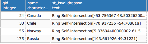
(4 rows)
      postgis_cookbook=# SELECT * INTO chp03.invalid_geometries FROM (
        SELECT 'broken'::varchar(10) as status,
        ST_GeometryN(the_geom, generate_series(
          1, ST_NRings(the_geom)))::geometry(Polygon,4326)
        as the_geom FROM chp03.countries
        WHERE name = 'Russia') AS foo
        WHERE ST_Intersects(the_geom,
          ST_SetSRID(ST_Point(143.661926,49.31221), 4326));
ST_MakeValid requires GEOS 3.3.0 or higher; check whether or not your system supports it using the PostGIS_full_version function as follows:
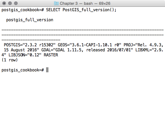
      postgis_cookbook=# INSERT INTO chp03.invalid_geometries
      VALUES ('repaired', (SELECT ST_MakeValid(the_geom)
      FROM chp03.invalid_geometries));

      postgis_cookbook=# SELECT status, ST_NRings(the_geom)
      FROM chp03.invalid_geometries;
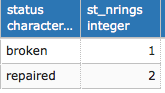
(2 rows)
      postgis_cookbook=# UPDATE chp03.countries
      SET the_geom = ST_MakeValid(the_geom)
      WHERE ST_IsValid(the_geom) = false;
There are a number of reasons why an invalid geometry could result in your database; for example, rings composed of polygons must be closed and cannot self-intersect or share more than one point with another ring.
After importing the country shapefile using the ST_IsValid and ST_IsValidReason functions, you will have figured out that four of the imported geometries are invalid, all because their polygons have self-intersecting rings.
At this point, a good way to investigate the invalid multipolygon geometry is by decomposing the polygon in to its component rings and checking out the invalid ones. For this purpose, we have exported the geometry of the ring causing the invalidity, using the ST_GeometryN function, which is able to extract the nth ring from the polygon. We coupled this function with the useful PostgreSQL generate_series function to iterate all of the rings composing the geometry, selecting the desired one using the ST_Intersects function.
As expected, the reason why this ring generates the invalidity is that it is self-intersecting and produces a hole in the polygon. While this adheres to the shapefile specification, it doesn't adhere to the OGC specification.
By running the ST_MakeValid function, PostGIS has been able to make the geometry valid, generating a second ring. Remember that the ST_MakeValid function is available only with the latest PostGIS compiled with the latest GEOS (3.3.0+). If that is not the setup for your working box and you cannot upgrade (upgrading is always recommended!), you can follow the techniques used in the past and discussed in a very popular, excellent presentation by Paul Ramsey at http://blog.opengeo.org/2010/09/08/tips-for-the-postgis-power-user/.
Joins for regular SQL tables have the real power in a relational database, and spatial joins are one of the most impressive features of a spatial database engine such as PostGIS.
Basically, it is possible to correlate information from different layers on the basis of the geometric relation of each feature from the input layers. In this recipe, we will take a tour of some common use cases of spatial joins.
$ ogrinfo 2012_Earthquakes_ALL.kml
The output for this is as follows:
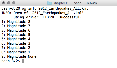
The following is the Linux version (name it import_eq.sh):
        #!/bin/bash
        for ((i = 1; i < 9 ; i++)) ; do
          echo "Importing earthquakes with magnitude $i
                to chp03.earthquakes PostGIS table..."
          ogr2ogr -append -f PostgreSQL -nln chp03.earthquakes
          PG:"dbname='postgis_cookbook' user='me'
          password='mypassword'" 2012_Earthquakes_ALL.kml
          -sql "SELECT name, description, CAST($i AS integer)
          AS magnitude FROM \"Magnitude $i\""
        done
The following is the Windows version (name it import_eq.bat):
        @echo off
        for /l %%i in (1, 1, 9) do (
          echo "Importing earthquakes with magnitude %%i
                to chp03.earthquakes PostGIS table..."
          ogr2ogr -append -f PostgreSQL -nln chp03.earthquakes
          PG:"dbname='postgis_cookbook' user='me'
          password='mypassword'" 2012_Earthquakes_ALL.kml
          -sql "SELECT name, description, CAST(%%i AS integer)
          AS magnitude FROM \"Magnitude %%i\""
        )
      $ chmod 775 import_eq.sh
      $ ./import_eq.sh
      Importing earthquakes with magnitude 1 to chp03.earthquakes
        PostGIS table...
      Importing earthquakes with magnitude 2 to chp03.earthquakes
        PostGIS table...
      ...
      postgis_cookbook=# ALTER TABLE chp03.earthquakes
      RENAME wkb_geometry  TO the_geom;
      $ ogr2ogr -f PostgreSQL -s_srs EPSG:4269 -t_srs EPSG:4326
      -lco GEOMETRY_NAME=the_geom -nln chp03.cities
      PG:"dbname='postgis_cookbook' user='me'
      password='mypassword'" citiesx020.shp
      $ ogr2ogr -f PostgreSQL -s_srs EPSG:4269 -t_srs EPSG:4326
      -lco GEOMETRY_NAME=the_geom -nln chp03.states -nlt MULTIPOLYGON
      PG:"dbname='postgis_cookbook' user='me'
      password='mypassword'" statesp020.shp
In this recipe, you will see for yourself the power of spatial SQL by solving a series of typical problems using spatial joins:
      postgis_cookbook=# SELECT s.state, COUNT(*) AS hq_count
      FROM chp03.states AS s
        JOIN chp03.earthquakes AS e
        ON ST_Intersects(s.the_geom, e.the_geom)
        GROUP BY s.state
        ORDER BY hq_count DESC;
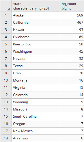
(33 rows)
      postgis_cookbook=# SELECT c.name, e.magnitude, count(*) as hq_count
      FROM chp03.cities AS c
        JOIN chp03.earthquakes AS e
        ON ST_DWithin(geography(c.the_geom), geography(e.the_geom), 200000)
        WHERE c.pop_2000 > 1000000
        GROUP BY c.name, e.magnitude
        ORDER BY c.name, e.magnitude, hq_count;
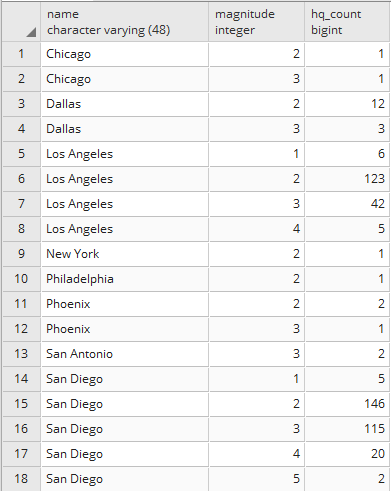
(18 rows)
      postgis_cookbook=# SELECT c.name, e.magnitude,
        ST_Distance(geography(c.the_geom), geography(e.the_geom))
      AS distance FROM chp03.cities AS c
        JOIN chp03.earthquakes AS e
        ON ST_DWithin(geography(c.the_geom), geography(e.the_geom), 200000)
        WHERE c.pop_2000 > 1000000
        ORDER BY distance;
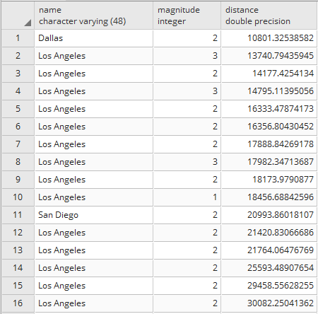
(488 rows)
      postgis_cookbook-# SELECT s.state, COUNT(*)
      AS city_count, SUM(pop_2000) AS pop_2000
      FROM chp03.states AS s
        JOIN chp03.cities AS c
        ON ST_Intersects(s.the_geom, c.the_geom)
        WHERE c.pop_2000 > 0 -- NULL values is -9999 on this field!
        GROUP BY s.state
        ORDER BY pop_2000 DESC;
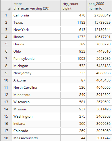
(51 rows)
      postgis_cookbook-# ALTER TABLE chp03.earthquakes
      ADD COLUMN state_fips character varying(2);
      postgis_cookbook-# UPDATE chp03.earthquakes AS e
        SET state_fips = s.state_fips
        FROM chp03.states AS s
        WHERE ST_Intersects(s.the_geom, e.the_geom);
Spatial joins are one of the key features that unleash the spatial power of PostGIS. For a regular join, it is possible to relate entities from two distinct tables using a common field. For a spatial join, it is possible to relate features from two distinct spatial tables using any spatial relationship function, such as ST_Contains, ST_Covers, ST_Crosses, and ST_DWithin.
In the first query, we used the ST_Intersects function to join the earthquake points to their respective state. We grouped the query by the state column to obtain the number of earthquakes in the state.
In the second query, we used the ST_DWithin function to relate each city to the earthquake points within a 200 km distance of it. We filtered out the cities with a population of less than 1 million inhabitants and grouped them by city name and earthquake magnitude to get a report of the number of earthquakes per city and by magnitude.
The third query is similar to the second one, except it doesn't group per city and by magnitude. The distance is computed using the ST_Distance function. Note that as feature coordinates are stored in WGS 84, you need to cast the geometric column to a spheroid and use the spheroid to get the distance in meters. Alternatively, you could project the geometries to a planar system that is accurate for the area we are studying in this recipe (in this case, the ESPG:2163, US National Atlas Equal Area would be a good choice) using the ST_Transform function. However, in the case of large areas like the one we've dealt with in this recipe, casting to geography is generally the best option as it gives more accurate results.
The fourth query uses the ST_Intersects function. In this case, we grouped by the state column and used two aggregation SQL functions (SUM and COUNT) to get the desired results.
Finally, in the last query, you update a spatial table using the results of a spatial join. The concept behind this is like that of the previous query, except that it is in the context of an UPDATE SQL command.
There will be many times when you will need to generate a less detailed and lighter version of a vector dataset, as you may not need very detailed features for several reasons. Think about a case where you are going to publish the dataset to a website and performance is a concern, or maybe you need to deploy the dataset to a colleague who does not need too much detail because they are using it for a large-area map. In all these cases, GIS tools include implementations of simplification algorithms that reduce unwanted details from a given dataset. Basically, these algorithms reduce the vertex numbers comprised in a certain tolerance, which is expressed in units measuring distance.
For this purpose, PostGIS provides you with the ST_Simplify and ST_SimplifyPreserveTopology functions. In many cases, they are the right solutions for simplification tasks, but in some cases, especially for polygonal features, they are not the best option out there and you will need a different GIS tool, such as GRASS or the new PostGIS topology support.
The steps you need to do to complete this recipe are as follows:
postgis_cookbook=# SET search_path TO chp03,public;
      postgis_cookbook=# CREATE TABLE states_simplify_topology AS
        SELECT ST_SimplifyPreserveTopology(ST_Transform(
          the_geom, 2163), 500) FROM states;
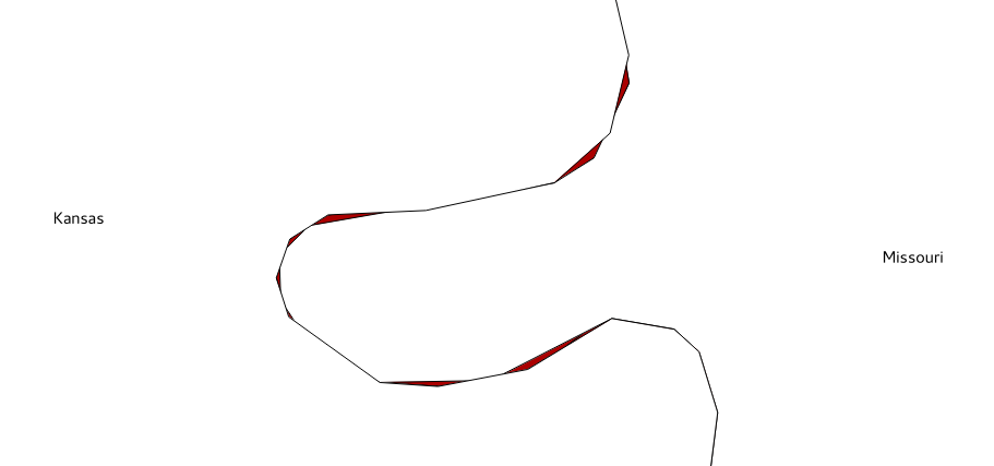
      SET search_path TO chp03, public;
      -- first project the spatial table to a planar system
        (recommended for simplification operations)
      CREATE TABLE states_2163 AS SELECT ST_Transform
        (the_geom, 2163)::geometry(MultiPolygon, 2163)
        AS the_geom, state FROM states;
      -- now decompose the geometries from multipolygons to polygons (2895)
        using the ST_Dump function
      CREATE TABLE polygons AS SELECT (ST_Dump(the_geom)).geom AS the_geom
        FROM states_2163;
      -- now decompose from polygons (2895) to rings (3150)
        using the ST_DumpRings function
      CREATE TABLE rings AS SELECT (ST_DumpRings(the_geom)).geom
        AS the_geom FROM polygons;
      -- now decompose from rings (3150) to linestrings (3150)
        using the ST_Boundary function
      CREATE TABLE ringlines AS SELECT(ST_boundary(the_geom))
        AS the_geom FROM rings;
      -- now merge all linestrings (3150) in a single merged linestring
        (this way duplicate linestrings at polygon borders disappear)
      CREATE TABLE mergedringlines AS SELECT ST_Union(the_geom)
        AS the_geom FROM ringlines;
      -- finally simplify the linestring with a tolerance of 150 meters
      CREATE TABLE simplified_ringlines AS SELECT
      ST_SimplifyPreserveTopology(the_geom, 150)
      AS the_geom FROM mergedringlines;
      -- now compose a polygons collection from the linestring
      using the ST_Polygonize function
      CREATE TABLE simplified_polycollection AS SELECT
        ST_Polygonize(the_geom) AS the_geom FROM simplified_ringlines;
      -- here you generate polygons (2895) from the polygons collection
        using ST_Dumps
      CREATE TABLE simplified_polygons AS SELECT
        ST_Transform((ST_Dump(the_geom)).geom,
        4326)::geometry(Polygon,4326)
        AS the_geom FROM simplified_polycollection;
      -- time to create an index, to make next operations faster
        CREATE INDEX simplified_polygons_gist ON simplified_polygons
        USING GIST (the_geom);
      -- now copy the state name attribute from old layer with a spatial
        join using the ST_Intersects and ST_PointOnSurface function
      CREATE TABLE simplified_polygonsattr AS SELECT new.the_geom,
        old.state FROM simplified_polygons new, states old
        WHERE ST_Intersects(new.the_geom, old.the_geom)
        AND ST_Intersects(ST_PointOnSurface(new.the_geom), old.the_geom);
      -- now make the union of all polygons with a common name
      CREATE TABLE states_simplified AS SELECT ST_Union(the_geom)
        AS the_geom, state FROM simplified_polygonsattr GROUP BY state;
$ mkdir grass_db
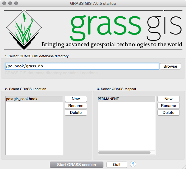
      GRASS 6.4.1 (postgis_cookbook):~ > v.in.ogr
      input=PG:"dbname='postgis_cookbook' user='me'
      password='mypassword'" layer=chp03.states_2163 out=states
GRASS 6.4.1 (postgis_cookbook):~ > v.info states
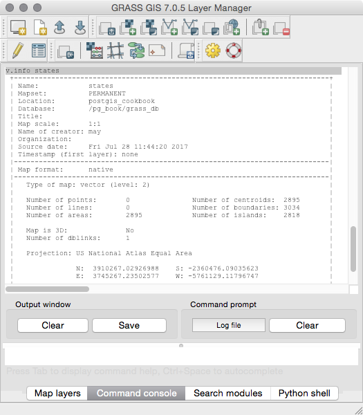
      GRASS 6.4.1 (postgis_cookbook):~ > v.generalize input=states
      output=states_generalized_from_grass method=douglas threshold=500
      GRASS 6.4.1 (postgis_cookbook):~ > v.out.ogr
      input=states_generalized_from_grass
      type=area dsn=PG:"dbname='postgis_cookbook' user='me'
      password='mypassword'" olayer=chp03.states_simplified_from_grass
      format=PostgreSQL
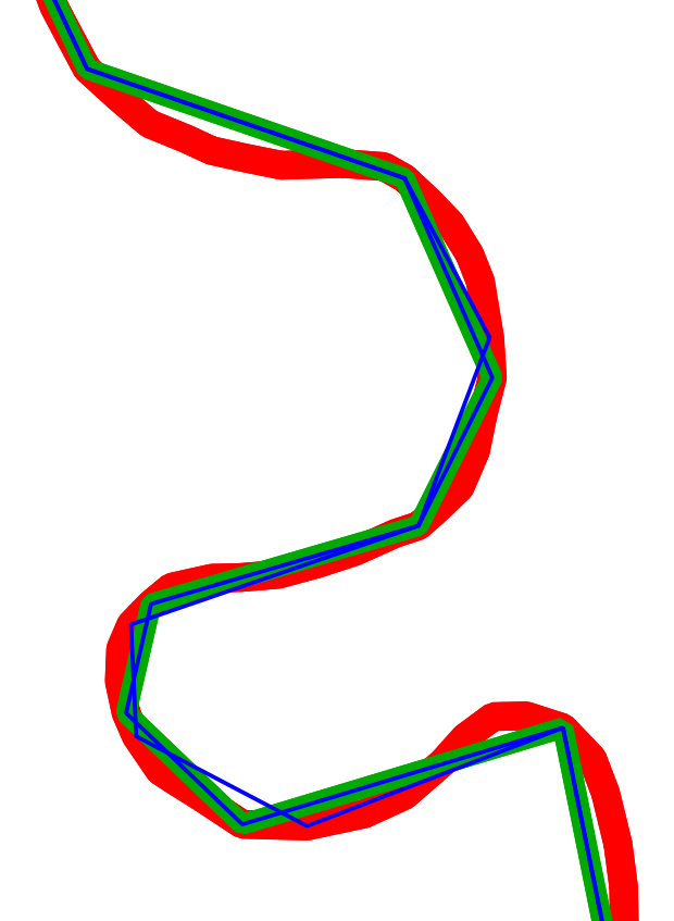
The ST_Simplify PostGIS function is able to simplify and generalize either a (simple or multi) linear or polygonal geometry using the Douglas-Peucker algorithm (for more details, go to http://en.wikipedia.org/wiki/Ramer%E2%80%93Douglas%E2%80%93Peucker_algorithm). Since it can create invalid geometries in some cases, it is recommended that you use its evolved version—the ST_SimplifyPreserveTopology function—which will produce only valid geometries.
While the functions are working well with (multi) linear geometries, in the case of (multi) polygons, they will most likely create topological anomalies such as overlaps and holes at shared polygon borders.
To get a valid, topologically simplified dataset, there are the following two choices at the time of writing:
While you will see the new PostGIS topological features in the Simplifying geometries with PostGIS topology recipe, in this one you have been using GRASS to perform the simplification process.
We opened GRASS, created a GIS data directory and a project location, and then imported in the GRASS location, the polygonal PostGIS table using the v.ogr.in command, based on GDAL/OGR as the name suggests.
Until this point, you have been using the GRASS v.generalize command to perform the simplification of the dataset using a tolerance (threshold) expressed in meters.
After simplifying the dataset, you imported it back to PostGIS using the v.ogr.out GRASS command and then opened the derived spatial table in a desktop GIS to see whether or not the process was performed in a topologically correct way.
In this recipe, we will check out the PostGIS functions needed for distance measurements (ST_Distance and its variants) and find out how considering the earth's curvature makes a big difference when measuring distances between distant points.
You should import the shapefile representing the cities from the USA that we generated in a previous recipe (the PostGIS table named chp03.cities). In case you haven't done so, download that shapefile from the https://nationalmap.gov/ website at http://dds.cr.usgs.gov/pub/data/nationalatlas/citiesx020_nt00007.tar.gz (this archive is also included in the code bundle available with this book) and import it to PostGIS:
$ ogr2ogr -f PostgreSQL -s_srs EPSG:4269 -t_srs EPSG:4326 -lco GEOMETRY_NAME=the_geom -nln chp03.cities PG:"dbname='postgis_cookbook' user='me' password='mypassword'" citiesx020.shp
The steps you need to perform to complete this recipe are as follows:
      postgis_cookbook=# SELECT c1.name, c2.name,
      ST_Distance(ST_Transform(c1.the_geom, 900913),
      ST_Transform(c2.the_geom, 900913))/1000 AS distance_900913
      FROM chp03.cities AS c1
      CROSS JOIN chp03.cities AS c2
      WHERE c1.pop_2000 > 1000000 AND c2.pop_2000 > 1000000
      AND c1.name < c2.name
      ORDER BY distance_900913 DESC;
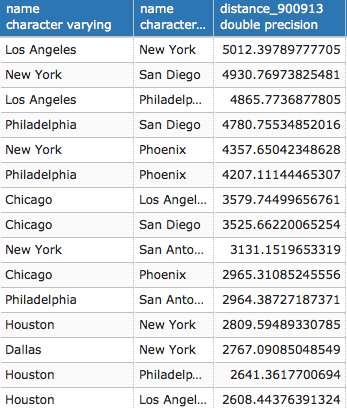
(36 rows)
      WITH cities AS (
        SELECT name, the_geom FROM chp03.cities
        WHERE pop_2000 > 1000000 )
      SELECT c1.name, c2.name,
      ST_Distance(ST_Transform(c1.the_geom, 900913),
      ST_Transform(c2.the_geom, 900913))/1000 AS distance_900913
      FROM cities c1 CROSS JOIN cities c2
      where c1.name < c2.name
      ORDER BY distance_900913 DESC;
      WITH cities AS (
        SELECT name, the_geom FROM chp03.cities
        WHERE pop_2000 > 1000000 )
      SELECT c1.name, c2.name,
      ST_Distance(ST_Transform(c1.the_geom, 900913),
      ST_Transform(c2.the_geom, 900913))/1000 AS d_900913,
      ST_Distance_Sphere(c1.the_geom, c2.the_geom)/1000 AS d_4326_sphere,
      ST_Distance_Spheroid(c1.the_geom, c2.the_geom,
      'SPHEROID["GRS_1980",6378137,298.257222101]')/1000
      AS d_4326_spheroid, ST_Distance(geography(c1.the_geom),
      geography(c2.the_geom))/1000 AS d_4326_geography
      FROM cities c1 CROSS JOIN cities c2
      where c1.name < c2.name
      ORDER BY d_900913 DESC;
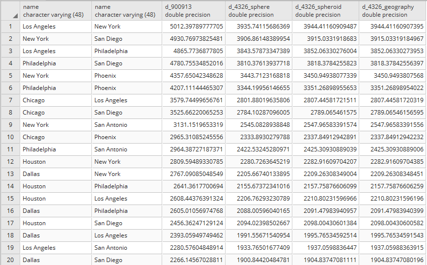
(36 rows)
If you need to compute the minimum Cartesian distance between two points, you can use the PostGIS ST_Distance function. This function accepts two-point geometries as input parameters and these geometries must be specified in the same spatial reference system.
If the two input geometries are using different spatial references, you can use the ST_Transform function on one or both of them to make them consistent with a single spatial reference system.
To get better results, you should consider the earth's curvature, which is mandatory when measuring large distances, and use the ST_Distance_Sphere or the ST_Distance_Spheroid functions. Alternatively, use ST_Distance, but cast the input geometries to the geography spatial data type, which is optimized for this kind of operation. The geography type stores the geometries in WGS 84 longitude latitude degrees, but it always returns the measurements in meters.
In this recipe, you have used a PostgreSQL CTE, which is a handy way to provide a subquery in the context of the main query. You can consider a CTE as a temporary table used only within the scope of the main query.
There are many cases in GIS workflows where you need to merge a polygonal dataset based on a common attribute. A typical example is merging the European administrative areas (which you can see at http://en.wikipedia.org/wiki/Nomenclature_of_Territorial_Units_for_Statistics), starting from Nomenclature des Units Territoriales Statistiques (NUTS) level 4 to obtain the subsequent levels up to NUTS level 1, using the NUTS code or merging the USA counties layer using the state code to obtain the states layer.
PostGIS lets you perform this kind of processing operation with the ST_Union function.
Download the USA countries shapefile from the https://nationalmap.gov/ website at http://dds.cr.usgs.gov/pub/data/nationalatlas/co2000p020_nt00157.tar.gz (this archive is also included in the code bundle provided with this book) and import it in PostGIS as follows:
$ ogr2ogr -f PostgreSQL -s_srs EPSG:4269 -t_srs EPSG:4326 -lco GEOMETRY_NAME=the_geom -nln chp03.counties -nlt MULTIPOLYGON PG:"dbname='postgis_cookbook' user='me' password='mypassword'" co2000p020.shp
The steps you need to perform to complete this recipe are as follows:
      postgis_cookbook=# SELECT county, fips, state_fips
      FROM chp03.counties ORDER BY county;
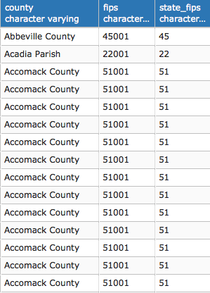
(6138 rows)
      postgis_cookbook=# CREATE TABLE chp03.states_from_counties
      AS SELECT ST_Multi(ST_Union(the_geom)) as the_geom, state_fips
      FROM chp03.counties GROUP BY state_fips;
You have been using the ST_Union PostGIS function to make a polygon merge on a common attribute. This function can be used as an aggregate PostgreSQL function (such as SUM, COUNT, MIN, and MAX) on the layer's geometric field, using the common attribute in the GROUP BY clause.
Note that ST_Union can also be used as a non-aggregate function to perform the union of two geometries (which are the two input parameters).
One typical GIS geoprocessing workflow is to compute intersections generated by intersecting linear geometries.
PostGIS offers a rich set of functions for solving this particular type of problem and you will have a look at them in this recipe.
For this recipe, we will use the Rivers + lake centerlines dataset of North America and Europe with a scale 1:10m. Download the rivers dataset from the following naturalearthdata.com website (or use the ZIP file included in the code bundle provided with this book):
Or find it on the following website:
http://www.naturalearthdata.com/downloads/10m-physical-vectors/
Extract the shapefile to your working directory chp03/working. Import the shapefile in PostGIS using shp2pgsql as follows:
$ shp2pgsql -I -W LATIN1 -s 4326 -g the_geom ne_10m_rivers_lake_centerlines.shp chp03.rivers > rivers.sql
$ psql -U me -d postgis_cookbook -f rivers.sql
The steps you need to perform to complete this recipe are as follows:
      postgis_cookbook=#  SELECT r1.gid AS gid1, r2.gid AS gid2,
      ST_AsText(ST_Intersection(r1.the_geom, r2.the_geom)) AS the_geom
      FROM chp03.rivers r1
      JOIN chp03.rivers r2
      ON ST_Intersects(r1.the_geom, r2.the_geom)
      WHERE r1.gid != r2.gid;
      postgis_cookbook=# SELECT COUNT(*),
        ST_GeometryType(ST_Intersection(r1.the_geom, r2.the_geom))
          AS geometry_type
        FROM chp03.rivers r1
        JOIN chp03.rivers r2
        ON ST_Intersects(r1.the_geom, r2.the_geom)
        WHERE r1.gid != r2.gid
        GROUP BY geometry_type;
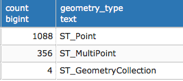
(3 rows)
      postgis_cookbook=# CREATE TABLE chp03.intersections_simple AS
        SELECT r1.gid AS gid1, r2.gid AS gid2,
          ST_Multi(ST_Intersection(r1.the_geom,
          r2.the_geom))::geometry(MultiPoint, 4326) AS the_geom
        FROM chp03.rivers r1
        JOIN chp03.rivers r2
        ON ST_Intersects(r1.the_geom, r2.the_geom)
        WHERE r1.gid != r2.gid
        AND ST_GeometryType(ST_Intersection(r1.the_geom,
          r2.the_geom)) != 'ST_GeometryCollection';
      postgis_cookbook=# CREATE TABLE chp03.intersections_all AS
      SELECT gid1, gid2, the_geom::geometry(MultiPoint, 4326) FROM (
        SELECT r1.gid AS gid1, r2.gid AS gid2,
        CASE
          WHEN ST_GeometryType(ST_Intersection(r1.the_geom,
            r2.the_geom)) != 'ST_GeometryCollection' THEN
          ST_Multi(ST_Intersection(r1.the_geom,
            r2.the_geom))
           ELSE ST_CollectionExtract(ST_Intersection(r1.the_geom,
            r2.the_geom), 1)
        END AS the_geom
        FROM chp03.rivers r1
        JOIN chp03.rivers r2
        ON ST_Intersects(r1.the_geom, r2.the_geom)
        WHERE r1.gid != r2.gid
      ) AS only_multipoints_geometries;
      postgis_cookbook=# SELECT SUM(ST_NPoints(the_geom))
        FROM chp03.intersections_simple; --2268 points per 1444 records
      postgis_cookbook=# SELECT SUM(ST_NPoints(the_geom))
        FROM chp03.intersections_all; --2282 points per 1448 records
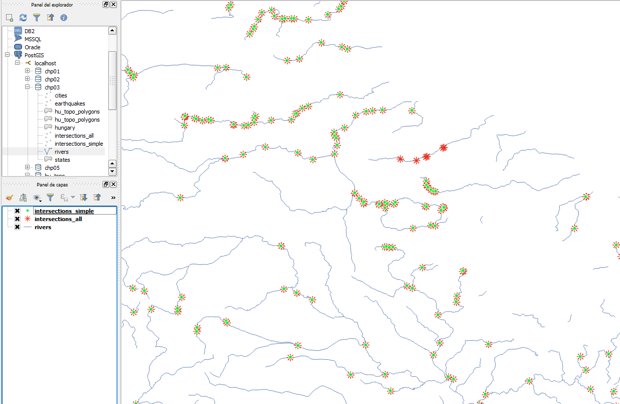
We have been using a self-spatial join of a linear PostGIS spatial layer to find intersections generated by the features of that layer.
To generate the self-spatial join, we used the ST_Intersects function. This way, we found that all of the features have at least an intersection in their respective geometries.
In the same self-spatial join context, we found out the intersections, using the ST_Intersection function.
The problem is that the computed intersections are not always single points. In fact, two intersecting lines can produce the origin for a single-point geometry (ST_Point) if the two lines just intersect once. But, the two intersecting lines can produce the origin for a point collection (ST_MultiPoint) or even a geometric collection if the two lines intersect at more points and/or share common parts.
As our target was to compute all the point intersections (ST_Point and ST_MultiPoint) using the ST_GeometryType function, we filtered out the values using a SQL SELECT CASE construct where the feature had a GeometryCollection geometry, for which we extracted just the points (and not the eventual linestrings) using the ST_CollectionExtract function (parameter type = 1) from the composing collections.
Finally, we compared the two result sets, both with plain SQL and a desktop GIS. The intersecting points computed filtered out the geometric collections from the output geometries and the intersecting points computed from all the geometries generated from the intersections, including the GeometryCollection features.
A common GIS use case is clipping a big dataset into small portions (subsets), with each perhaps representing an area of interest. In this recipe, you will export from a PostGIS layer representing the rivers in the world, with one distinct shapefile composed of rivers for each country. For this purpose, you will use the ST_Intersection function.
Be sure that you have imported in PostGIS the same river dataset (a shapefile) that was used in the previous recipe.
The steps you need to take to complete this recipe are as follows:
       postgis_cookbook=> CREATE VIEW chp03.rivers_clipped_by_country AS
         SELECT r.name, c.iso2, ST_Intersection(r.the_geom,
           c.the_geom)::geometry(Geometry,4326) AS the_geom
         FROM chp03.countries AS c
         JOIN chp03.rivers AS r
         ON ST_Intersects(r.the_geom, c.the_geom);
mkdir working/chp03/rivers
The following is the Linux version (name it export_rivers.sh):
        #!/bin/bash
        for f in `ogrinfo PG:"dbname='postgis_cookbook' user='me'
        password='mypassword'" -sql "SELECT DISTINCT(iso2)
        FROM chp03.countries ORDER BY iso2" | grep iso2 | awk '{print $4}'`
        do
          echo "Exporting river shapefile for $f country..."
          ogr2ogr rivers/rivers_$f.shp PG:"dbname='postgis_cookbook'
          user='me' password='mypassword'"
          -sql "SELECT * FROM chp03.rivers_clipped_by_country
          WHERE iso2 = '$f'"
        done
The following is the Windows version (name it export_rivers.bat):
        FOR /F "tokens=*" %%f IN ('ogrinfo
        PG:"dbname=postgis_cookbook user=me password=password"
        -sql "SELECT DISTINCT(iso2) FROM chp03.countries
         ORDER BY iso2" ^| grep iso2 ^| gawk "{print $4}"') DO (
           echo "Exporting river shapefile for %%f country..."
           ogr2ogr rivers/rivers_%%f.shp PG:"dbname='postgis_cookbook'
           user='me' password='password'"
           -sql "SELECT * FROM chp03.rivers_clipped_by_country
           WHERE iso2 = '%%f'"
        )
C:\export_rivers.bat
      $ chmod 775 export_rivers.sh
      $ ./export_rivers.sh
      Exporting river shapefile for AD country...
      Exporting river shapefile for AE country...
      ...
      Exporting river shapefile for ZM country...
      Exporting river shapefile for ZW country...
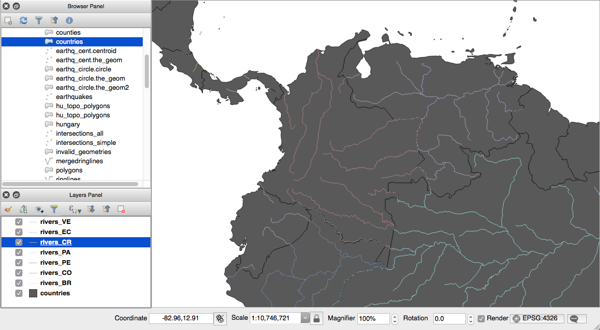
You can use the ST_Intersection function to clip one dataset from another. In this recipe, you first created a view, where you performed a spatial join between a polygonal layer (countries) and a linear layer (rivers) using the ST_Intersects function. In the context of the spatial join, you have used the ST_Intersection function to generate a snapshot of the rivers in every country.
You have then created a bash script in which you iterated every single country and pulled out to a shapefile the clipped rivers for that country, using ogr2ogr and the previously created view as the input layer.
To iterate the countries in the script, you have been using ogrinfo with the -sql option, using a SQL SELECT DISTINCT statement. You have used a combination of the grep and awk Linux commands, piped together to get every single country code. The grep command is a utility for searching plaintext datasets for lines matching a regular expression, while awk is an interpreted programming language designed for text processing and typically used as a data extraction and reporting tool.
In a previous recipe, we used the ST_SimplifyPreserveTopology function to try to generate a simplification of a polygonal PostGIS layer.
Unfortunately, while that function works well for linear layers, it produces topological anomalies (overlapping and holes) in shared polygon borders. You used an external toolset (GRASS) to generate a valid topological simplification.
In this recipe, you will use the PostGIS topology support to perform the same task within the spatial database, without needing to export the dataset to a different toolset.
To get started, perform the following steps:
postgis_cookbook=# CREATE EXTENSION postgis_topology;
      ogr2ogr -f PostgreSQL -t_srs EPSG:3857 -nlt MULTIPOLYGON
      -lco GEOMETRY_NAME=the_geom -nln chp03.hungary
      PG:"dbname='postgis_cookbook' user='me'
      password='mypassword'" HUN_adm1.shp
postgis_cookbook=# SELECT COUNT(*) FROM chp03.hungary;

(1 row)
The steps you need to take to complete this recipe are as follows:
postgis_cookbook=# SET search_path TO chp03, topology, public;
postgis_cookbook=# SELECT CreateTopology('hu_topo', 3857);
postgis_cookbook=# SELECT * FROM topology.topology;
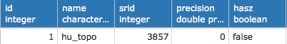
(1 rows)
postgis_cookbook=# \dtv hu_topo.*
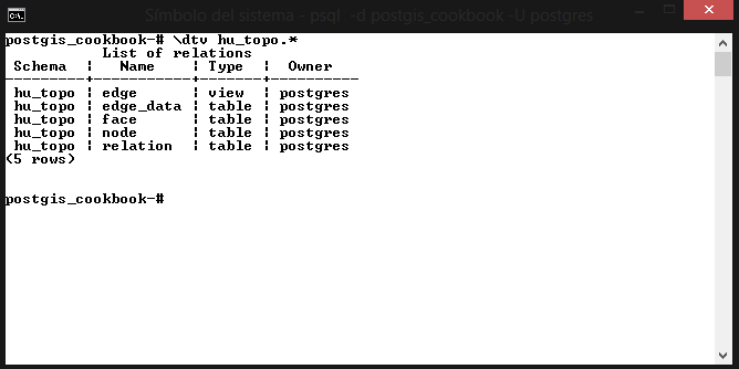
(5 rows)
postgis_cookbook=# SELECT topologysummary('hu_topo');
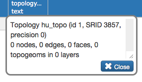
(1 row)
      postgis_cookbook=# CREATE TABLE
        chp03.hu_topo_polygons(gid serial primary key, name_1 varchar(75));
      postgis_cookbook=# SELECT
        AddTopoGeometryColumn('hu_topo', 'chp03', 'hu_topo_polygons',
       'the_geom_topo', 'MULTIPOLYGON') As layer_id;
      postgis_cookbook=> INSERT INTO
      chp03.hu_topo_polygons(name_1, the_geom_topo)
        SELECT name_1, toTopoGeom(the_geom, 'hu_topo', 1)
        FROM chp03.hungary;
        Query returned successfully: 20 rows affected,
                                     10598 ms execution time.
postgis_cookbook=# SELECT topologysummary('hu_topo');
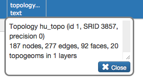
      postgis_cookbook=# SELECT row_number() OVER
      (ORDER BY ST_Area(mbr) DESC) as rownum, ST_Area(mbr)/100000
      AS area FROM hu_topo.face ORDER BY area DESC;
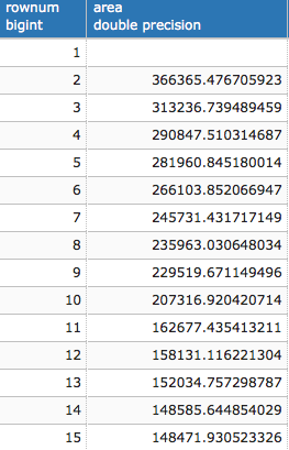
(93 rows)
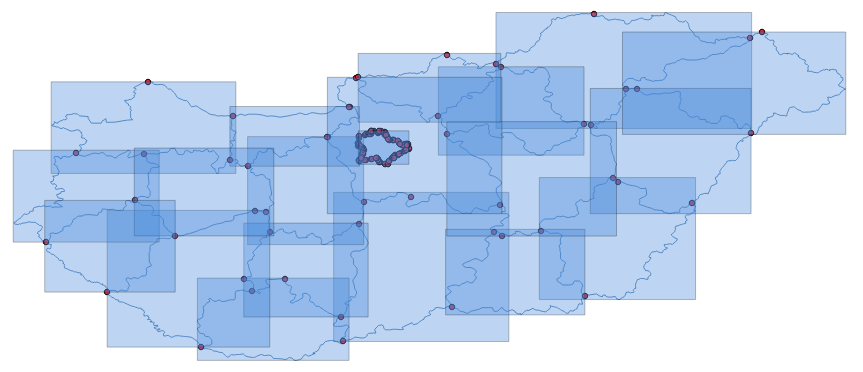
      postgis_cookbook=# SELECT DropTopology('hu_topo');
      postgis_cookbook=# DROP TABLE chp03.hu_topo_polygons;
      postgis_cookbook=# SELECT CreateTopology('hu_topo', 3857, 1);
      postgis_cookbook=# CREATE TABLE chp03.hu_topo_polygons(
        gid serial primary key, name_1 varchar(75));
      postgis_cookbook=# SELECT AddTopoGeometryColumn('hu_topo',
        'chp03', 'hu_topo_polygons', 'the_geom_topo',
        'MULTIPOLYGON') As layer_id;
      postgis_cookbook=# INSERT INTO
      chp03.hu_topo_polygons(name_1, the_geom_topo)
        SELECT name_1, toTopoGeom(the_geom, 'hu_topo', 1)
        FROM chp03.hungary;
postgis_cookbook=# SELECT topologysummary('hu_topo');
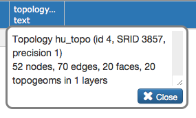
(1 row)
      postgis_cookbook=# SELECT ST_ChangeEdgeGeom('hu_topo',
        edge_id, ST_SimplifyPreserveTopology(geom, 500))
        FROM hu_topo.edge;
      postgis_cookbook=# UPDATE chp03.hungary hu
        SET the_geom = hut.the_geom_topo
        FROM chp03.hu_topo_polygons hut
        WHERE hu.name_1 = hut.name_1;
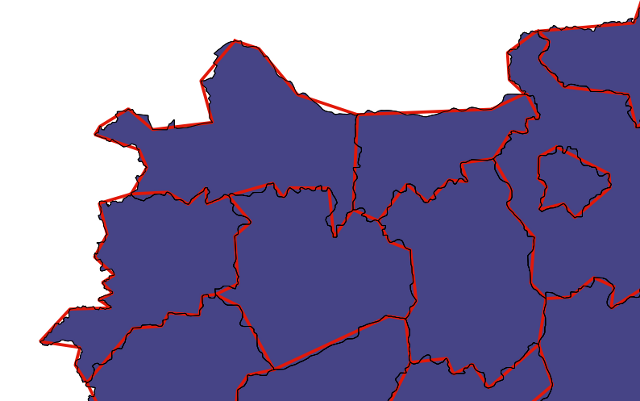
We created a new PostGIS topology schema using the CreateTopology function. This function creates a new PostgreSQL schema where all the topological entities are stored.
We can have more topological schemas within the same spatial database, each being contained in a different PostgreSQL schema. The PostGIS topology.topology table manages all the metadata for all the topological schemas.
Each topological schema is composed of a series of tables and views to manage the topological entities (such as edge, edge data, face, node, and topogeoms) and their relations.
We can have a quick look at the description of a single topological schema using the topologysummary function, which summarizes the main metadata information-name, SRID, and precision; the number of nodes, edges, faces, topogeoms, and topological layers; and, for each topological layer, the geometry type, and the number of topogeoms.
After creating the topology schema, we created a new PostGIS table and added to it a topological geometry column (topogeom in PostGIS topology jargon) using the AddTopoGeometryColumn function.
We then used the ST_ChangeEdgeGeom function to alter the geometries for the topological edges, using the ST_SimplifyPreserveTopology function, with a tolerance of 500 meters, and checked that this function, used in the context of a topological schema, produces topologically correct results for polygons too.
In this chapter, we will cover:
Beyond being a spatial database with the capacity to store and query spatial data, PostGIS is a very powerful analytical tool. What this means to the user is a tremendous capacity to expose and encapsulate deep spatial analyses right within a PostgreSQL database.
The recipes in this chapter can roughly be divided into four main sections:
The basic question that we seek to answer in this recipe is the fundamental distance question, which are the five coffee shops closest to me? It turns out that while it is a fundamental question, it's not always easy to answer, though we will make this possible in this recipe. We will approach this in two steps. The first step with which we'll approach this is in a simple heuristic way, which will allow us to come to a solution quickly. Then, we'll take advantage of the deeper PostGIS functionality to make the solution faster and more general with a k-Nearest Neighbor (KNN) approach.
A concept that we need to understand from the outset is that of a spatial index. A spatial index, like other database indexes, functions like a book index. It is a special construct to make looking for things inside our table easier, much in the way a book index helps us find content in a book faster. In the case of a spatial index, it helps us find faster ways, when things are in space. Therefore, by using a spatial index in our geographic searches, we can speed up our searches by orders of magnitude.
We will start by loading our data. Our data is the address records from Cuyahoga County, Ohio, USA:
shp2pgsql -s 3734 -d -i -I -W LATIN1 -g the_geom CUY_ADDRESS_POINTS chp04.knn_addresses | psql -U me -d postgis_cookbook
As this dataset may take a while to load, you can alternatively load a subset:
shp2pgsql -s 3734 -d -i -I -W LATIN1 -g the_geom CUY_ADDRESS_POINTS_subset chp04.knn_addresses | psql -U me -d postgis_cookbook
We specified the -I flag in order to request that a spatial index be created upon the import of this data.
Let us start by seeing how many records we are dealing with:
SELECT COUNT(*) FROM chp04.knn_addresses;
--484958
We have, in this address table, almost half a million address records, which is not an insubstantial number to perform a query.
KNN is an approach of searching for an arbitrary number of points closest to a given point. Without the right tools, this can be a very slow process that requires testing the distance between the point of interest and all the possible neighbors. The problem with this approach is that the search becomes exponentially slower with a greater number of points. Let's start with this naive approach and then improve on it.
Suppose we were interested in finding the 10 records closest to the geographic location -81.738624, 41.396679. The naive approach would be to transform this value into our local coordinate system and compare the distance to each point in the database from the search point, order those values by distance, and limit the search to the first 10 closest records (it is not recommended that you run the following query as it could run indefinitely):
SELECT ST_Distance(searchpoint.the_geom, addr.the_geom) AS dist, * FROM
  chp04.knn_addresses addr,
  (SELECT ST_Transform(ST_SetSRID(ST_MakePoint(-81.738624, 41.396679),
    4326), 3734) AS the_geom) searchpoint
  ORDER BY ST_Distance(searchpoint.the_geom, addr.the_geom)
  LIMIT 10;
This is a fine approach for smaller datasets. This is a logical, simple, fast approach for a relatively small numbers of records; however, this approach scales very poorly, getting exponentially slower with the addition of records (with 500,000 points, this would take a very long time).
An alternative is to only compare the point of interest to the ones known to be close by setting a search distance. So, for example, in the following diagram, we have a star that represents the current location, and we want to know the 10 closest addresses. The grid in the diagram is 100 feet long, so we can search for the points within 200 feet, then measure the distance to each of these points, and return the closest 10 points:
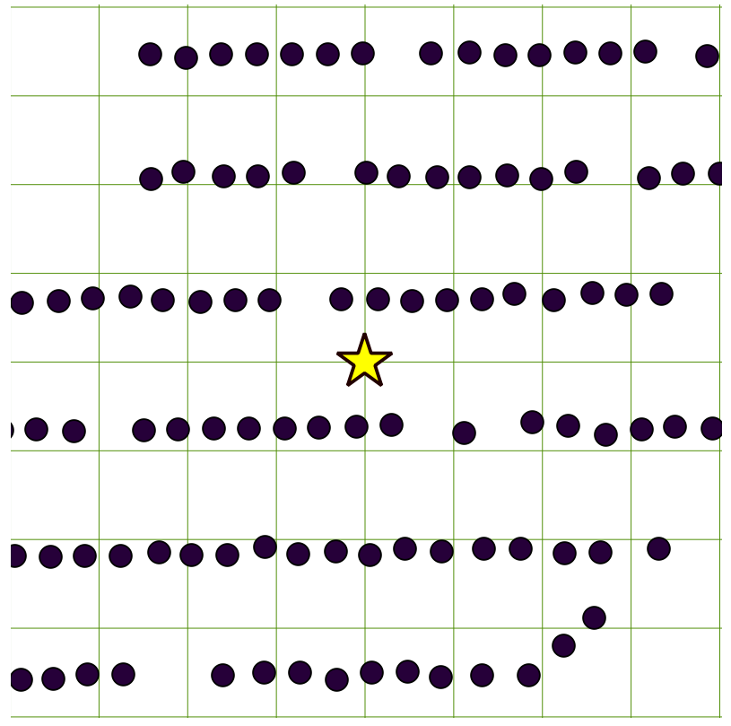
Thus, our approach to answer this question is to limit the search using the ST_DWithin operator to only search for records within a certain distance. ST_DWithin uses our spatial index, so the initial distance search is fast and the list of returned records should be short enough to do the same pair-wise distance comparison we did earlier in this section. In our case here, we could limit the search to within 200 feet:
SELECT ST_Distance(searchpoint.the_geom, addr.the_geom) AS dist, * FROM
  chp04.knn_addresses addr,
  (SELECT ST_Transform(ST_SetSRID(ST_MakePoint(-81.738624, 41.396679),
    4326), 3734) AS the_geom) searchpoint
  WHERE ST_DWithin(searchpoint.the_geom, addr.the_geom, 200)
  ORDER BY ST_Distance(searchpoint.the_geom, addr.the_geom)
  LIMIT 10;
The output for the previous query is as follows:
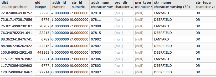
This approach performs well so long as our search window, ST_DWithin, is the right size for the data. The problem with this approach is that, in order to optimize it, we need to know how to set a search window that is about the right size. Any larger than the right size and the query will run more slowly than we'd like. Any smaller than the right size and we might not get all the points back that we need. Inherently, we don't know this ahead of time, so we can only hope for the best guess.
In this same dataset, if we apply the same query in another location, the output will return no points because the 10 closest points are further than 200 feet away. We can see this in the following diagram:
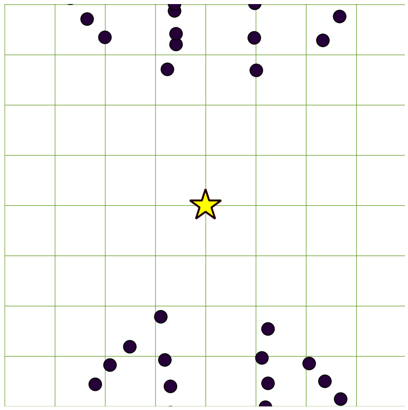
Fortunately, for PostGIS 2.0+ we can leverage the distance operators (<-> and <#>) to do indexed nearest neighbor searches. This makes for very fast KNN searches that don't require us to guess ahead of time how far away we need to search. Why are the searches fast? The spatial index helps of course, but in the case of the distance operator, we are using the structure of the index itself, which is hierarchical, to very quickly sort our neighbors.
When used in an ORDER BY clause, the distance operator uses the index:
SELECT ST_Distance(searchpoint.the_geom, addr.the_geom) AS dist, * FROM
  chp04.knn_addresses addr,
  (SELECT ST_Transform(ST_SetSRID(ST_MakePoint(-81.738624, 41.396679),
    4326), 3734) AS the_geom) searchpoint
  ORDER BY addr.the_geom <-> searchpoint.the_geom
  LIMIT 10;
This approach requires no prior knowledge of how far the nearest neighbors might be. It also scales very well, returning thousands of records in not more than the time it takes to return a few records. It is sometimes slower than using ST_DWithin, depending on how small our search distance is and how large the dataset we are dealing with is. But the trade-off is that we don't need to make a guess of our search distance and for large queries, it can be much faster than the naive approach.
What makes this magic possible is that PostGIS uses an R-tree index. This means that the index itself is sorted hierarchically based on spatial information. As demonstrated, we can leverage the structure of the index in sorting distances from a given arbitrary location, and thus use the index to directly return the sorted records. This means that the structure of the spatial index itself helps us answer such fundamental questions quickly and inexpensively.
In the preceding recipe, we wanted to answer the simple question of which are the nearest 10 locations to a given point. There is another simple question with a surprisingly sophisticated answer. The question is how do we approach this problem when we want to traverse an entire dataset and test each record for its nearest neighbors?
Our problem is as follows: for each point in our table, we are interested in the angle to the nearest object in another table. A case demonstrating this scenario is if we want to represent address points as building-like squares rotated to align with an adjacent road, similar to the historic United States Geological Survey (USGS) quadrangle maps, as shown in the following screenshot:

For larger buildings, USGS quads show the buildings' footprints, but for residential buildings below their minimum threshold, the points are just rotated squares—a nice cartographic effect that could easily be replicated with address points.
As in the previous recipe, we will start off by loading our data. Our data is the address records from Cuyahoga County, Ohio, USA. If you loaded this in the previous recipe, there is no need to reload the data. If you have not loaded the data yet, run the following command:
shp2pgsql -s 3734 -d -i -I -W LATIN1 -g the_geom CUY_ADDRESS_POINTS chp04.knn_addresses | psql -U me -d postgis_cookbook
As this dataset may take a while to load, you can alternatively load a subset using the following command:
shp2pgsql -s 3734 -d -i -I -W LATIN1 -g the_geom CUY_ADDRESS_POINTS_subset chp04.knn_addresses | psql -U me -d postgis_cookbook
The address points will serve as a proxy for our building structures. However, to align our structure to the nearby streets, we will need a streets layer. We will use Cuyahoga County's street centerline data for this:
shp2pgsql -s 3734 -d -i -I -W LATIN1 -g the_geom CUY_STREETS chp04.knn_streets | psql -U me -d postgis_cookbook
Before we commence, we have to consider another aspect of using indexes, which we didn't need to consider in our previous KNN recipe. When our KNN approach used only points, our indexing was exact—the bounding box of a point is effectively a point. As bounding boxes are what indexes are built around, our indexing estimates of distance perfectly reflected the actual distances between our points. In the case of non-point geometries, as is our example here, the bounding box is an approximation of the lines to which we will be comparing our points. Put another way, what this means is that our nearest neighbor may not be our very nearest neighbor, but is likely our approximate nearest neighbor, or one of our nearest neighbors.
In practice, we apply a heuristic approach: we simply gather slightly more than the number of nearest neighbors we are interested in and then sort them based on the actual distance in order to gather only the number we are interested in. In this way, we only need to sort a small number of records.
Insofar as KNN is a nuanced approach to these problems, forcing KNN to run on all the records in a dataset takes what I like to call a venerable and age-old approach. In other words, it requires a bit of a hack.
In SQL, the typical way to loop is to use a SELECT statement. For our case, we don't have a function that does KNN looping through the records in a table to use; we simply have an operator that allows us to efficiently order our returning records by distance from a given record. The workaround is to write a temporary function and thus be able to use SELECT to loop through the records for us. The cost is the creation and deletion of the function, plus the work done by the query, and the combination of costs is well worth the hackiness of the approach.
First, consider the following function:
CREATE OR REPLACE FUNCTION chp04.angle_to_street (geometry) RETURNS double precision AS $$

WITH index_query as (SELECT ST_Distance($1,road.the_geom) as dist, degrees(ST_Azimuth($1, ST_ClosestPoint(road.the_geom, $1))) as azimuth FROM  chp04.knn_streets As road ORDER BY $1 <#> road.the_geom limit 5)

SELECT azimuth FROM index_query ORDER BY dist
LIMIT 1;

$$ LANGUAGE SQL;
Now, we can use this function quite easily:
CREATE TABLE chp04.knn_address_points_rot AS SELECT addr.*, chp04.angle_to_street(addr.the_geom) FROM chp04.knn_addresses addr;
If you have loaded the whole address dataset, this will take a while.
If we choose to, we can optionally drop the function so that extra functions are not left in our database:
DROP FUNCTION chp04.angle_to_street (geometry);
In the next recipe, Rotating geometries, the calculated angle will be used to build new geometries.
Our function is simple, KNN magic aside. As an input to the function, we allow geometry, as shown in the following query:
CREATE OR REPLACE FUNCTION chp04.angle_to_street (geometry) RETURNS double precision AS $$
The preceding function returns a floating-point value.
We then use a WITH statement to create a temporary table, which returns the five closest lines to our point of interest. Remember, as the index uses bounding boxes, we don't really know which line is the closest, so we gather a few extra points and then filter them based on distance. This idea is implemented in the following query:
WITH index_query as (SELECT ST_Distance($1,road.geom) as dist, degrees(ST_Azimuth($1, ST_ClosestPoint(road.geom, $1))) as azimuth
FROM street_centerlines As road
ORDER BY $1 <#> road.geom LIMIT 5)
Note that we are actually returning to columns. The first column is dist, in which we calculate the distance to the nearest five road lines. Note that this operation is performed after the ORDER BY and LIMIT functions have been used as filters, so this does not take much computation. Then, we use ST_Azimuth to calculate the angle from our point to the closest points (ST_ClosestPoint) on each of our nearest five lines. In summary, what returns with our temporary index_query table is the distance to the nearest five lines and the respective rotation angles to the nearest five lines.
If we recall, however, we were not looking for the angle to the nearest five but to the true nearest road line. For this, we order the results by distance and further use LIMIT 1:
SELECT azimuth FROM index_query ORDER BY dist
LIMIT 1;
Among the many functions that PostGIS provides, geometry manipulation is a very powerful addition. In this recipe, we will explore a simple example of using the ST_Rotate function to rotate geometries. We will use a function from the Improving proximity filtering with KNN – advanced recipe to calculate our rotation values.
ST_Rotate has a few variants: ST_RotateX, ST_RotateY, and ST_RotateZ, with the ST_Rotate function serving as an alias for ST_RotateZ. Thus, for two-dimensional cases, ST_Rotate is a typical use case.
In the Improving proximity filtering with KNN – advanced recipe, our function calculated the angle to the nearest road from a building's centroid or address point. We can symbolize that building's point according to that rotation factor as a square symbol, but more interestingly, we can explicitly build the area of that footprint in real space and rotate it to match our calculated rotation angle.
Recall our function from the Improving proximity filtering with KNN – advanced recipe:
CREATE OR REPLACE FUNCTION chp04.angle_to_street (geometry) RETURNS double precision AS $$

WITH index_query as (SELECT ST_Distance($1,road.the_geom) as dist, degrees(ST_Azimuth($1, ST_ClosestPoint(road.the_geom, $1))) as azimuth
FROM  chp04.knn_streets As road
ORDER BY $1 <#> road.the_geom limit 5)

SELECT azimuth FROM index_query ORDER BY dist
LIMIT 1;

$$ LANGUAGE SQL;
This function will calculate the geometry's angle to the nearest road line. Now, to construct geometries using this calculation, run the following function:
CREATE TABLE chp04.tsr_building AS

SELECT ST_Rotate(ST_Envelope(ST_Buffer(the_geom, 20)), radians(90 - chp04.angle_to_street(addr.the_geom)), addr.the_geom)
  AS the_geom FROM chp04.knn_addresses addr
LIMIT 500;
In the first step, we are taking each of the points and first applying a buffer of 20 feet to them:
ST_Buffer(the_geom, 20)
Then, we calculate the envelope of the buffer, providing us with a square around that buffered area. This is a quick and easy way to create a square geometry of a specified size from a point:
ST_Envelope(ST_Buffer(the_geom, 20))
Finally, we use ST_Rotate to rotate the geometry to the appropriate angle. Here is where the query becomes harder to read. The ST_Rotate function takes two arguments:
ST_Rotate(geometry to rotate, angle, origin around which to rotate)
The geometry we are using is the newly calculated geometry from the buffering and envelope creation. The angle is the one we calculate using our chp04.angle_to_street function. Finally, the origin around which we rotate is the input point itself, resulting in the following portion of our query:
ST_Rotate(ST_Envelope(ST_Buffer(the_geom, 20)), radians(90 -chp04.angle_to_street(addr.the_geom)), addr.the_geom);
This gives us some really nice cartography, as shown in the following diagram:
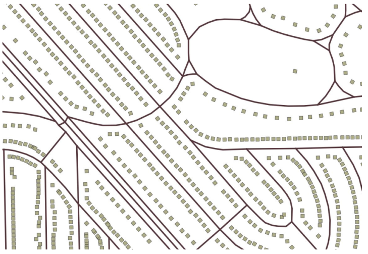
In this short recipe, we will be using a common coding pattern in use when geometries are being constructed with ST_Polygonize and formalizing it into a function for reuse.
ST_Polygonize is a very useful function. You can pass a set of unioned lines or an array of lines to ST_Polygonize, and the function will construct polygons from the input. ST_Polygonize does so aggressively insofar as it will construct all possible polygons from the inputs. One frustrating aspect of the function is that it does not return a multi-polygon, but instead returns a geometry collection. Geometry collections can be problematic in third-party tools for interacting with PostGIS as so many third party tools don't have mechanisms in place for recognizing and displaying geometry collections.
The pattern we will formalize here is the commonly recommended approach for changing geometry collections into mutlipolygons when it is appropriate to do so. This approach will be useful not only for ST_Polygonize, which we will use in the subsequent recipe, but can also be adapted for other cases where a function returns geometry collections, which are, for all practical purposes, multi-polygons. Hence, this is why it merits its own dedicated recipe.
The basic pattern for handling geometry collections is to use ST_Dump to convert them to a dump type, extract the geometry portion of the dump, collect the geometry, and then convert this collection into a multi-polygon. The dump type is a special PostGIS type that is a combination of the geometries and an index number for the geometries. It's typical to use ST_Dump to convert from a geometry collection to a dump type and then do further processing on the data from there. Rarely is a dump object used directly, but it is typically an intermediate type of data.
We expect this function to take a geometry and return a multi-polygon geometry:
CREATE OR REPLACE FUNCTION chp04.polygonize_to_multi (geometry) RETURNS geometry AS $$
For readability, we will use a WITH statement to construct the series of transformations in geometry. First, we will polygonize:
WITH polygonized AS (
  SELECT ST_Polygonize($1) AS the_geom
),
Then, we will dump:
dumped AS (
  SELECT (ST_Dump(the_geom)).geom AS the_geom FROM polygonized
)
Now, we can collect and construct a multi-polygon from our result:
SELECT ST_Multi(ST_Collect(the_geom)) FROM dumped;
Put this together into a single function:
CREATE OR REPLACE FUNCTION chp04.polygonize_to_multi (geometry) RETURNS geometry AS $$

WITH polygonized AS (
  SELECT ST_Polygonize($1) AS the_geom
),
dumped AS (
  SELECT (ST_Dump(the_geom)).geom AS the_geom FROM polygonized
)
SELECT ST_Multi(ST_Collect(the_geom)) FROM dumped;
$$ LANGUAGE SQL;
Now, we can polygonize directly from a set of closed lines and skip the typical intermediate step when we use the ST_Polygonize function of having to handle a geometry collection.
Often, in a spatial database, we are interested in making explicit the representation of geometries that are implicit in the data. In the example that we will use here, the explicit portion of the geometry is a single point coordinate where a field survey plot has taken place. In the following screenshot, this explicit location is the dot. The implicit geometry is the actual extent of the field survey, which includes 10 subplots arranged in a 5 x 2 array and rotated according to a bearing.
These subplots are the purple squares in the following diagram:
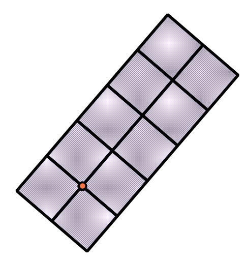
There are a number of ways for us to approach this problem. In the interest of simplicity, we will first construct our grid and then rotate it in place. Also, we could in principle use a ST_Buffer function in combination with ST_Extent to construct the squares in our resultant geometry, but, as ST_Extent uses floating-point approximations of the geometry for the sake of efficiency, this could result in some mismatches at the edges of our subplots.
The approach we will use for the construction of the subplots is to construct the grid with a series of ST_MakeLine and use ST_Node to flatten or node the results. This ensures that we have all of our lines properly intersecting each other. ST_Polygonize will then construct our multi-polygon geometry for us. We will leverage this function through our wrapper function from the Improving ST_Polygonize recipe.
Our plots are 10 units on a side, in a 5 x 2 array. As such, we can imagine a function to which we pass our plot origin, and the function returns a multi-polygon of all the subplot geometries. One additional element to consider is that the orientation of the layout of our plots is rotated to a bearing. We expect the function to actually use two inputs, so origin and rotation will be the variables that we will pass to our function.
We can consider geometry and a float value as the inputs, and we want the function to return geometry:
CREATE OR REPLACE FUNCTION chp04.create_grid (geometry, float) RETURNS geometry AS $$
In order to construct the subplots, we will require three lines running parallel to the X axis:
WITH middleline AS (
  SELECT ST_MakeLine(ST_Translate($1, -10, 0),
    ST_Translate($1, 40.0, 0)) AS the_geom
),
topline AS (
  SELECT ST_MakeLine(ST_Translate($1, -10, 10.0),
    ST_Translate($1, 40.0, 10)) AS the_geom
),
bottomline AS (
  SELECT ST_MakeLine(ST_Translate($1, -10, -10.0),
    ST_Translate($1, 40.0, -10)) AS the_geom
),
And we will require six lines running parallel to the Y axis:
oneline AS (
  SELECT ST_MakeLine(ST_Translate($1, -10, 10.0),
    ST_Translate($1, -10, -10)) AS the_geom
),
twoline AS (
  SELECT ST_MakeLine(ST_Translate($1, 0, 10.0),
    ST_Translate($1, 0, -10)) AS the_geom
),
threeline AS (
  SELECT ST_MakeLine(ST_Translate($1, 10, 10.0),
    ST_Translate($1, 10, -10)) AS the_geom
),
fourline AS (
  SELECT ST_MakeLine(ST_Translate($1, 20, 10.0),
    ST_Translate($1, 20, -10)) AS the_geom
),
fiveline AS (
  SELECT ST_MakeLine(ST_Translate($1, 30, 10.0),
    ST_Translate($1, 30, -10)) AS the_geom
),
sixline AS (
  SELECT ST_MakeLine(ST_Translate($1, 40, 10.0),
    ST_Translate($1, 40, -10)) AS the_geom
),
To use these for polygon construction, we will require them to have nodes where they cross and touch. A UNION ALL function will combine these lines in a single record; ST_Union will provide the geometric processing necessary to construct the nodes of interest and will combine our lines into a single entity ready for chp04.polygonize_to_multi:
combined AS (
  SELECT ST_Union(the_geom) AS the_geom FROM
  (
    SELECT the_geom FROM middleline
      UNION ALL
    SELECT the_geom FROM topline
      UNION ALL
    SELECT the_geom FROM bottomline
      UNION ALL
    SELECT the_geom FROM oneline
      UNION ALL
    SELECT the_geom FROM twoline
      UNION ALL
    SELECT the_geom FROM threeline
      UNION ALL
    SELECT the_geom FROM fourline
      UNION ALL
    SELECT the_geom FROM fiveline
      UNION ALL
    SELECT the_geom FROM sixline
  ) AS alllines
)
But we have not created polygons yet, just lines. The final step, using our polygonize_to_multi function, finishes the work for us:
SELECT chp04.polygonize_to_multi(ST_Rotate(the_geom, $2, $1)) AS the_geom FROM combined;
The combined query is as follows:
CREATE OR REPLACE FUNCTION chp04.create_grid (geometry, float) RETURNS geometry AS $$

WITH middleline AS (
  SELECT ST_MakeLine(ST_Translate($1, -10, 0),
    ST_Translate($1, 40.0, 0)) AS the_geom
),
topline AS (
  SELECT ST_MakeLine(ST_Translate($1, -10, 10.0),
    ST_Translate($1, 40.0, 10)) AS the_geom
),
bottomline AS (
  SELECT ST_MakeLine(ST_Translate($1, -10, -10.0),
    ST_Translate($1, 40.0, -10)) AS the_geom
),
oneline AS (
  SELECT ST_MakeLine(ST_Translate($1, -10, 10.0),
    ST_Translate($1, -10, -10)) AS the_geom
),
twoline AS (
  SELECT ST_MakeLine(ST_Translate($1, 0, 10.0),
    ST_Translate($1, 0, -10)) AS the_geom
),
threeline AS (
  SELECT ST_MakeLine(ST_Translate($1, 10, 10.0),
    ST_Translate($1, 10, -10)) AS the_geom
),
fourline AS (
  SELECT ST_MakeLine(ST_Translate($1, 20, 10.0),
    ST_Translate($1, 20, -10)) AS the_geom
),
fiveline AS (
  SELECT ST_MakeLine(ST_Translate($1, 30, 10.0),
    ST_Translate($1, 30, -10)) AS the_geom
),
sixline AS (
  SELECT ST_MakeLine(ST_Translate($1, 40, 10.0),
    ST_Translate($1, 40, -10)) AS the_geom
),
combined AS (
  SELECT ST_Union(the_geom) AS the_geom FROM
  (
    SELECT the_geom FROM middleline
      UNION ALL
    SELECT the_geom FROM topline
      UNION ALL
    SELECT the_geom FROM bottomline
      UNION ALL
    SELECT the_geom FROM oneline
      UNION ALL
    SELECT the_geom FROM twoline
      UNION ALL
    SELECT the_geom FROM threeline
      UNION ALL
    SELECT the_geom FROM fourline
      UNION ALL
    SELECT the_geom FROM fiveline
      UNION ALL
    SELECT the_geom FROM sixline
  ) AS alllines
)
SELECT chp04.polygonize_to_multi(ST_Rotate(the_geom, $2, $1)) AS the_geom FROM combined;
$$ LANGUAGE SQL;
This function, shown in the preceding section, essentially draws the geometry from a single input point and rotation value. It does so by using nine instances of ST_MakeLine. Typically, one might use ST_MakeLine in combination with ST_MakePoint to accomplish this. We bypass this need by having the function consume a point geometry as an input. We can, therefore, use ST_Translate to move this point geometry to the endpoints of the lines of interest in order to construct our lines with ST_MakeLine.
One final step, of course, is to test the use of our new geometry constructing function:
CREATE TABLE chp04.tsr_grid AS

-- embed inside the function
  SELECT chp04.create_grid(ST_SetSRID(ST_MakePoint(0,0),
  3734), 0) AS the_geom
    UNION ALL
  SELECT chp04.create_grid(ST_SetSRID(ST_MakePoint(0,100),
  3734), 0.274352 * pi()) AS the_geom
    UNION ALL
  SELECT chp04.create_grid(ST_SetSRID(ST_MakePoint(100,0),
  3734), 0.824378 * pi()) AS the_geom
    UNION ALL
  SELECT chp04.create_grid(ST_SetSRID(ST_MakePoint(0,-100), 3734),
  0.43587 * pi()) AS the_geom
    UNION ALL
  SELECT chp04.create_grid(ST_SetSRID(ST_MakePoint(-100,0), 3734),
  1 * pi()) AS the_geom;
The different grids generated by the previous functions are the following:

Frequently, with spatial analyses, we receive data in one form that seems quite promising but we need it in another more extensive form. LiDAR is an excellent solution for such problems; LiDAR data is laser scanned either from an airborne platform, such as a fixed-wing plane or helicopter, or from a ground unit. LiDAR devices typically return a cloud of points referencing absolute or relative positions in space. As a raw dataset, they are often not as useful as they are once they have been processed. Many LiDAR datasets are classified into land cover types, so a LiDAR dataset, in addition to having data that contains x, y, and z values for all the points sampled across a space, will often contain LiDAR points that are classified as ground, vegetation, tall vegetation, buildings, and so on.
As useful as this is, the data is intensive, that is, it has discreet points, rather than extensive, as polygon representations of such data would be. This recipe was developed as a simple method to use PostGIS to transform the intensive LiDAR samples of buildings into extensive building footprints:
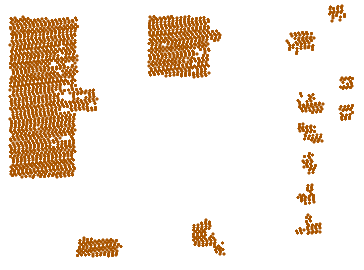
The LiDAR dataset we will use is a 2006 collection, which was classified into ground, tall vegetation (> 20 feet), buildings, and so on. One characteristic of the analysis that follows is that we assume the classification to be correct, and so we are not revisiting the quality of the classification or attempting to improve it within PostGIS.
A characteristic of the LiDAR dataset is that a sample point exists for relatively flat surfaces at approximately no fewer than 1 for every 5 feet. This will inform you about how we manipulate the data.
First, let's load our dataset using the following command:
shp2pgsql -s 3734 -d -i -I -W LATIN1 -g the_geom lidar_buildings chp04.lidar_buildings | psql -U me -d postgis_cookbook
The simplest way to convert point data to polygon data would be to buffer the points by their known separation:
ST_Buffer(the_geom, 5)
We can imagine, however, that such a simplistic approach might look strange:
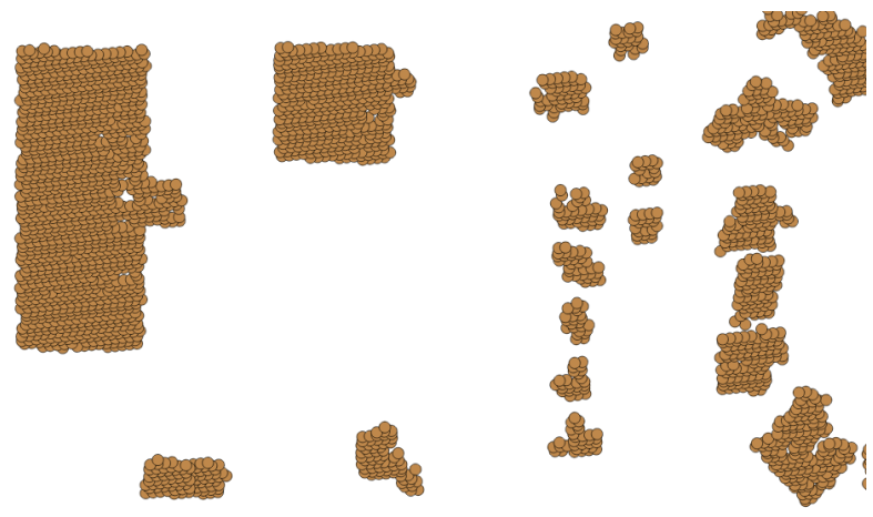
As such, it would be good to perform a union of these geometries in order to dissolve the internal boundaries:
ST_Union(ST_Buffer(the_geom, 5))
Now, we can see the start of some simple building footprints:
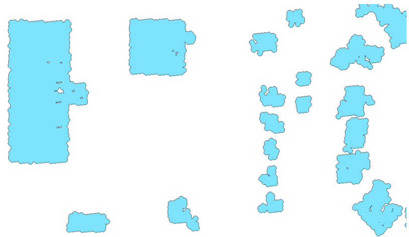
While this is marginally better, the result is quite lumpy. We will use the ST_Simplify_PreserveTopology function to simplify the polygons and then grab just the external ring to remove the internal holes:
CREATE TABLE chp04.lidar_buildings_buffer AS

WITH lidar_query AS
(SELECT ST_ExteriorRing(ST_SimplifyPreserveTopology(
  (ST_Dump(ST_Union(ST_Buffer(the_geom, 5)))).geom, 10
)) AS the_geom FROM chp04.lidar_buildings)

SELECT chp04.polygonize_to_multi(the_geom) AS the_geom from lidar_query;
Now, we have simplified versions of our buffered geometries:

There are two things to note here. The larger the building, relative to the density of the sampling, the better it looks. We might query to eliminate smaller buildings, which are likely to degenerate when this approach is used, depending on the density of our LiDAR data.
To put it informally, our buffering technique effectively lumps together or clusters adjacent samples. This is possible only because we have regularly sampled data, but that is OK. The density and scan patterns for the LiDAR data are typical of such datasets, so we can expect this approach to be applicable to other datasets.
The ST_Union function converts these discreet buffered points into a single record with dissolved internal boundaries. To complete the clustering, we simply need to use ST_Dump to convert these boundaries back to discreet polygons so that we can utilize individual building footprints. Finally, we simplify the pattern with ST_SimplifyPreserveTopology and extract the external ring, or use ST_ExteriorRing outside these polygons, which removes the holes inside the building footprints. Since ST_ExteriorRing returns a line, we have to reconstruct our polygon. We use chp04.polygonize_to_multi, a function we wrote in the Improving ST_Polygonize recipe, to handle just such occasions. In addition, you can check the Normalizing internal overlays recipe in Chapter 2, Structures That Work, in order to learn how to correct polygons with possible geographical errors.
In PostGIS version 2.3, some cluster functionalities were introduced. In this recipe, we will explore ST_ClusterKMeans, a function that aggregates geometries into k clusters and retrieves the id of the assigned cluster for each geometry in the input. The general syntax for the function is as follows:
ST_ClusterKMeans(geometry winset geom, integer number_of_clusters);
In this recipe, we will use the earthquake dataset included in the source from Chapter 3, Working with Vector Data – The Basics, as our input geometries for the function. We also need to define the number of clusters that the function will output; the value of k for this example will be 10. You could play with this value and see the different cluster arrangements the function outputs; the greater the value for k, the smaller the number of geometries each cluster will contain.
If you have not previously imported the earthquake data into the Chapter 3, Working with Vector Data – The Basics, schema, refer to the Getting ready section of the GIS analysis with spatial joins recipe.
Once we have created the chp03.earthquake table, we will need two tables. The first one will contain the centroid geometries of the clusters and their respective IDs, which the ST_ClusterKMeans function retrieves. The second table will have the geometries for the minimum bounding circle for each cluster. To do so, run the following SQL commands:
CREATE TABLE chp04.earthq_cent (
  cid integer PRIMARY KEY, the_geom geometry('POINT',4326)
);

CREATE TABLE chp04.earthq_circ (
  cid integer PRIMARY KEY, the_geom geometry('POLYGON',4326)
);
We will then populate the centroid table by generating the cluster ID for each geometry in chp03.earthquakes using the ST_ClusterKMeans function, and then we will use the ST_Centroid function to calculate the 10 centroids for each cluster:
INSERT INTO chp04.earthq_cent (the_geom, cid) (
  SELECT DISTINCT ST_SetSRID(ST_Centroid(tab2.ge2), 4326) as centroid,
  tab2.cid FROM(
    SELECT ST_UNION(tab.ge) OVER (partition by tab.cid ORDER BY tab.cid)
    as ge2, tab.cid as cid FROM(
      SELECT ST_ClusterKMeans(e.the_geom, 10) OVER() AS cid, e.the_geom
      as ge FROM chp03.earthquakes as e) as tab
  )as tab2
);
If we check the inserted rows with the following command:
SELECT * FROM chp04.earthq_cent;
The output will be as follows:
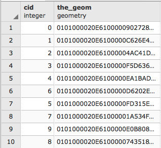
Then, insert the corresponding minimum bounding circles for the clusters in the chp04.earthq_circ table. Execute the following SQL command:
# INSERT INTO chp04.earthq_circ (the_geom, cid) (
  SELECT DISTINCT ST_SetSRID(
    ST_MinimumBoundingCircle(tab2.ge2), 4326) as circle, tab2.cid
    FROM(
      SELECT ST_UNION(tab.ge) OVER (partition by tab.cid ORDER BY tab.cid)
      as ge2, tab.cid as cid
      FROM(
        SELECT ST_ClusterKMeans(e.the_geom, 10) OVER() as cid, e.the_geom
        as ge FROM chp03.earthquakes AS e
      ) as tab
    )as tab2
  );
In a desktop GIS, import all three tables as layers (chp03.earthquakes, chp04.earthq_cent, and chp04.earthq_circ) in order to visualize them and understand the clustering. Note that circles may overlap; however, this does not mean that clusters do as well, since each point belongs to one and only one cluster, but the minimum bounding circle for a cluster may overlap with another minimum bounding circle for another cluster:
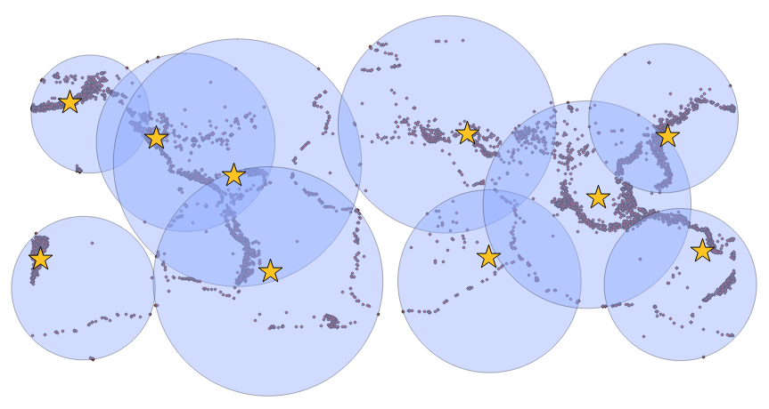
In the 2.3 version, PostGIS provides a way to create Voronoi diagrams from the vertices of a geometry; this will work only with versions of GEOS greater than or equal to 3.5.0.
The following is a Voronoi diagram generated from a set of address points. Note how the points from which the diagram was generated are equidistant to the lines that divide them. Packed soap bubbles viewed from above form a similar network of shapes:
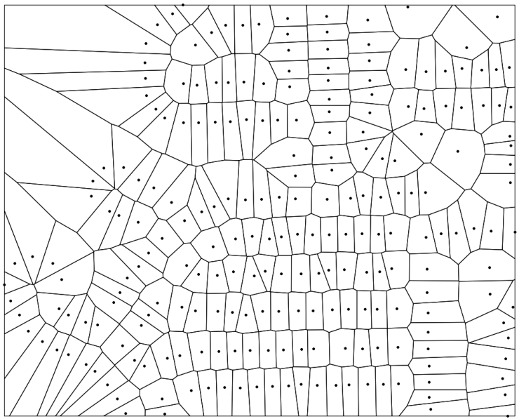
Voronoi diagrams are a space-filling approach that are useful for a variety of spatial analysis problems. We can use these to create space filling polygons around points, the edges of which are equidistant from all the surrounding points.
The PostGIS function ST_VoronoiPolygons(), receives the following parameters: a geometry from which to build the Voronoi diagram, a tolerance, which is a float that will tell the function the distance within which vertices will be treated as equivalent for the output, and an extent_to geometry that will tell the extend of the diagram if this geometry is bigger than the calculated output from the input vertices. For this recipe, we will not use tolerance, which defaults to 0.0 units, nor extend_to, which is set to NULL by default.
We will create a small arbitrary point dataset to feed into our function around which we will calculate the Voronoi diagram:
DROP TABLE IF EXISTS chp04.voronoi_test_points;
CREATE TABLE chp04.voronoi_test_points
(
  x numeric,
  y numeric
)
WITH (OIDS=FALSE);

ALTER TABLE chp04.voronoi_test_points ADD COLUMN gid serial;
ALTER TABLE chp04.voronoi_test_points ADD PRIMARY KEY (gid);

INSERT INTO chp04.voronoi_test_points (x, y)
  VALUES (random() * 5, random() * 7);
INSERT INTO chp04.voronoi_test_points (x, y)
  VALUES (random() * 2, random() * 8);
INSERT INTO chp04.voronoi_test_points (x, y)
  VALUES (random() * 10, random() * 4);
INSERT INTO chp04.voronoi_test_points (x, y)
  VALUES (random() * 1, random() * 15);
INSERT INTO chp04.voronoi_test_points (x, y)
  VALUES (random() * 4, random() * 9);
INSERT INTO chp04.voronoi_test_points (x, y)
  VALUES (random() * 8, random() * 3);
INSERT INTO chp04.voronoi_test_points (x, y)
  VALUES (random() * 5, random() * 3);
INSERT INTO chp04.voronoi_test_points (x, y)
  VALUES (random() * 20, random() * 0.1);
INSERT INTO chp04.voronoi_test_points (x, y)
  VALUES (random() * 5, random() * 7);

SELECT AddGeometryColumn ('chp04','voronoi_test_points','the_geom',3734,'POINT',2);

UPDATE chp04.voronoi_test_points
  SET the_geom = ST_SetSRID(ST_MakePoint(x,y), 3734)
  WHERE the_geom IS NULL
;
With preparations in place, now we are ready to create the Voronoi diagram. First, we will create the table that will contain the MultiPolygon:
DROP TABLE IF EXISTS chp04.voronoi_diagram;
CREATE TABLE chp04.voronoi_diagram(
  gid serial PRIMARY KEY,
  the_geom geometry(MultiPolygon, 3734)
);
Now, to calculate the Voronoi diagram, we use ST_Collect in order to provide a MultiPoint object for the ST_VoronoiPolygons function. The output of this alone would be a GeometryCollection; however, we are interested in getting a MultiPolygon instead, so we need to use the ST_CollectionExtract function, which when given the number 3 as the second parameter, extracts all polygons from a GeometryCollection:
INSERT INTO chp04.voronoi_diagram(the_geom)(
  SELECT ST_CollectionExtract(
    ST_SetSRID(
      ST_VoronoiPolygons(points.the_geom),
    3734),
  3)
  FROM (
    SELECT
    ST_Collect(the_geom) as the_geom
    FROM chp04.voronoi_test_points
  )
as points);
If we import the layers for voronoi_test_points and voronoi_diagram into a desktop GIS, we get the following Voronoi diagram of the randomly generated points:
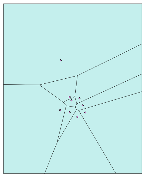
Now we can process much larger datasets. The following is a Voronoi diagram derived from the address points from the Improving proximity filtering with KNN – advanced recipe, with the coloration based on the azimuth to the nearest street, also calculated in that recipe:
In this chapter, we will cover the following:
In this chapter, the recipes are presented in a step-by-step workflow that you may apply while working with a raster. This entails loading the raster, getting a basic understanding of the raster, processing and analyzing it, and delivering it to consumers. We intentionally add some detours to the workflow to reflect the reality that the raster, in its original form, may be confusing and not suitable for analysis. At the end of this chapter, you should be able to take the lessons learned from the recipes and confidently apply them to solve your raster problems.
Before going further, we should describe what a raster is, and what a raster is used for. At the simplest level, a raster is a photo or image with information describing where to place the raster on the Earth's surface. A photograph typically has three sets of values: one set for each primary color (red, green, and blue). A raster also has sets of values, often more than those found in a photograph. Each set of values is known as a band. So, a photograph typically has three bands, while a raster has at least one band. Like digital photographs, rasters come in a variety of file formats. Common raster formats you may come across include PNG, JPEG, GeoTIFF, HDF5, and NetCDF. Since rasters can have many bands and even more values, they can be used to store large quantities of data in an efficient manner. Due to their efficiency, rasters are used for satellite and aerial sensors and modeled surfaces, such as weather forecasts.
There are a few keywords used in this chapter and in the PostGIS ecosystem that need to be defined:
We make heavy use of GDAL in this chapter. GDAL is generally considered the de facto Swiss Army knife for working with rasters. GDAL is not a single application, but is a raster-abstraction library with many useful utilities. Through GDAL, you can get the metadata of a raster, convert that raster to a different format, and warp that raster among many other capabilities. For our needs in this chapter, we will use three GDAL utilities: gdalinfo, gdalbuildvrt, and gdal_translate.
In this recipe, we load most of the rasters used in this chapter. These rasters are examples of satellite imagery and model-generated surfaces, two of the most common raster sources.
If you have not done so already, create a directory and copy the chapter's datasets; for Windows, use the following commands:
> mkdir C:\postgis_cookbook\data\chap05
> cp -r /path/to/book_dataset/chap05 C:\postgis_cookbook\data\chap05
For Linux or macOS, go into the folder you wish to use and run the following commands, where /path/to/book_dataset/chap05 is the path where you originally stored the book source code:
> mkdir -p data/chap05
> cd data/chap05
> cp -r /path/to/book_dataset/chap05
You should also create a new schema for this chapter in the database:
> psql -d postgis_cookbook -c "CREATE SCHEMA chp05"
We will start with the PRISM average monthly minimum-temperature raster dataset for 2016 with coverage for the continental United States. The raster is provided by the PRISM Climate Group at Oregon State University, with additional rasters available at http://www.prism.oregonstate.edu/mtd/.
On the command line, navigate to the PRISM directory as follows:
> cd C:\postgis_cookbook\data\chap05\PRISM
Let us spot check one of the PRISM rasters with the GDAL utility gdalinfo. It is always a good practice to inspect at least one raster to get an idea of the metadata and ensure that the raster does not have any issues. This can be done using the following command:
> gdalinfo PRISM_tmin_provisional_4kmM2_201703_asc.asc
The gdalinfo output is as follows:
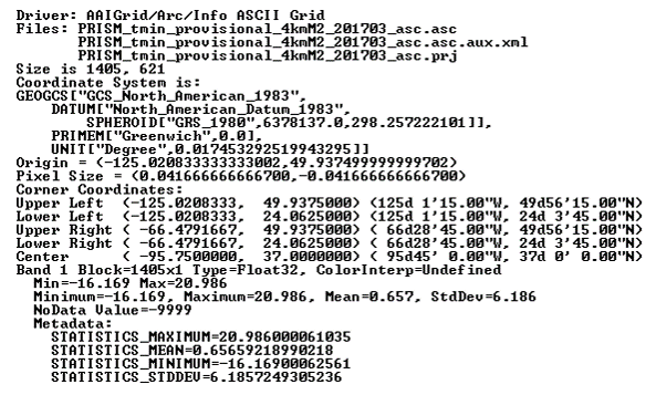
The gdalinfo output reveals that the raster has no issues, as evidenced by the Corner Coordinates, Pixel Size, Band, and Coordinate System being unempty.
Looking through the metadata, we find that the metadata about the spatial reference system indicates that raster uses the NAD83 coordinate system. We can double-check this by searching for the details of NAD83 in the spatial_ref_sys table:
SELECT srid, auth_name, auth_srid, srtext, proj4text
FROM spatial_ref_sys WHERE proj4text LIKE '%NAD83%'
Comparing the text of srtext to the PRISM raster's metadata spatial attributes, we find that the raster is in EPSG (SRID 4269).
You can load the PRISM rasters into the chp05.prism table with raster2pgsql, which will import the raster files to the database in a similar manner as the shp2pgsql command:
> raster2pgsql -s 4269 -t 100x100 -F -I -C -Y .\PRISM_tmin_provisional_4kmM2_*_asc.asc
chp05.prism | psql -d postgis_cookbook -U me
The raster2pgsql command is called with the following flags:
There is a reason why we passed -F to raster2pgsql. If you look at the filenames of the PRISM rasters, you'll note the year and month. So, let's convert the value in the filename column to a date in the table:
ALTER TABLE chp05.prism ADD COLUMN month_year DATE;
UPDATE chp05.prism SET  month_year = ( SUBSTRING(split_part(filename, '_', 5), 0, 5) || '-' ||  SUBSTRING(split_part(filename, '_', 5), 5, 4) || '-01' ) :: DATE;
This is all that needs to be done with the PRISM rasters for now.
Now, let's import a Shuttle Radar Topography Mission (SRTM) raster. The SRTM raster is from the SRTM that was conducted by the NASA Jet Propulsion Laboratory in February, 2000. This raster and others like it are available at: http://dds.cr.usgs.gov/srtm/version2_1/SRTM1/.
Change the current directory to the SRTM directory:
> cd C:\postgis_cookbook\data\chap05\SRTM
Make sure you spot check the SRTM raster with gdalinfo to ensure that it is valid and has a value for Coordinate System. Once checked, import the SRTM raster into the chp05.srtm table:
> raster2pgsql -s 4326 -t 100x100 -F -I -C -Y N37W123.hgt chp05.srtm | psql -d postgis_cookbook
We use the same raster2pgsql flags for the SRTM raster as those for the PRISM rasters.
We also need to import a shapefile of San Francisco provided by the City and County of San Francisco, available with the book's dataset files, or the one found on the following link, after exporting the data to a shapefile:
https://data.sfgov.org/Geographic-Locations-and-Boundaries/SF-Shoreline-and-Islands/rgcx-5tix
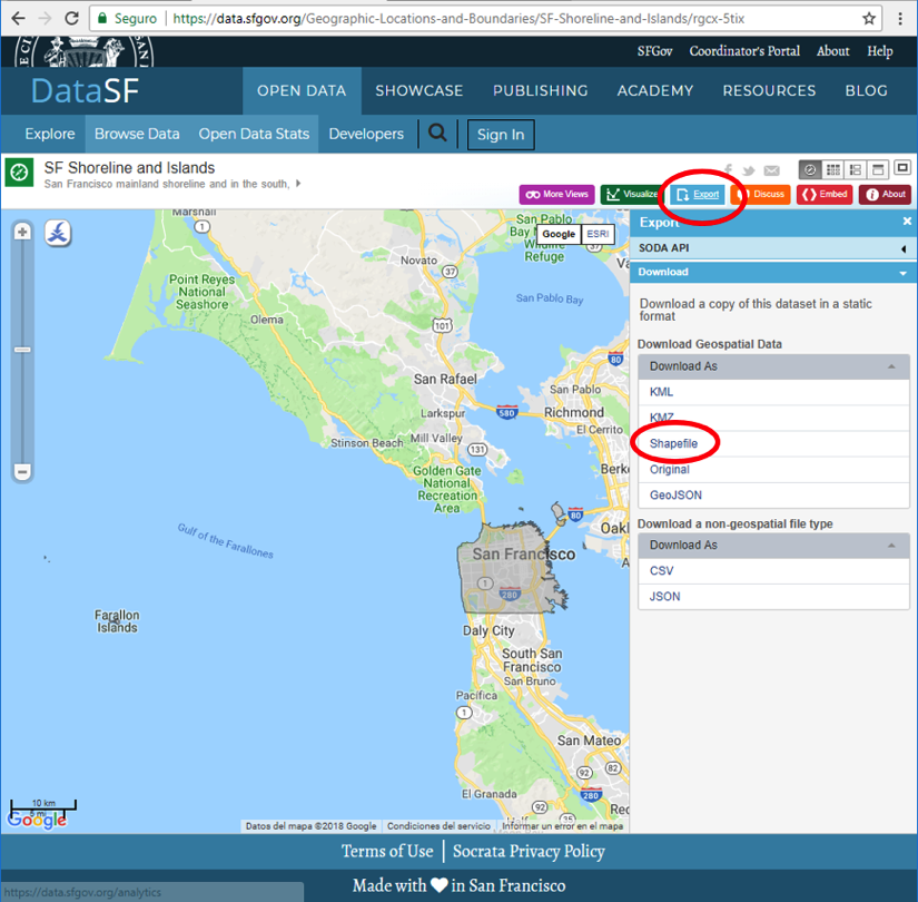
The San Francisco's boundaries from the book's files will be used in many of the follow-up recipes, and it must be loaded to the database as follows:
> cd C:\postgis_cookbook\data\chap05\SFPoly
> shp2pgsql -s 4326 -I sfpoly.shp chp05.sfpoly | psql -d postgis_cookbook -U me
In this recipe, we imported the required PRISM and SRTM rasters needed for the rest of the recipes. We also imported a shapefile containing San Francisco's boundaries to be used in the various raster analyses. Now, on to the fun!
So far, we've checked and imported the PRISM and SRTM rasters into the chp05 schema of the postgis_cookbook database. We will now proceed to work with the rasters within the database.
In this recipe, we explore functions that provide insight into the raster attributes and characteristics found in the postgis_cookbook database. In doing so, we can see if what is found in the database matches the information provided by accessing gdalinfo.
PostGIS includes the raster_columns view to provide a high-level summary of all the raster columns found in the database. This view is similar to the geometry_columns and geography_columns views in function and form.
Let's run the following SQL query in the raster_columns view to see what information is available in the prism table:
SELECT
  r_table_name,
  r_raster_column,
  srid,
  scale_x,
  scale_y,
  blocksize_x,
  blocksize_y,
  same_alignment,
  regular_blocking,
  num_bands,
  pixel_types,
  nodata_values,
  out_db,
  ST_AsText(extent) AS extent FROM raster_columns WHERE r_table_name = 'prism';
The SQL query returns a record similar to the following:


(1 row)
If you look back at the gdalinfo output for one of the PRISM rasters, you'll see that the values for the scales (the pixel size) match. The flags passed to raster2pgsql, specifying tile size and SRID, worked.
Let's see what the metadata of a single raster tile looks like. We will use the ST_Metadata() function:
SELECT rid, (ST_Metadata(rast)).* FROM chp05.prism WHERE month_year = '2017-03-01'::date LIMIT 1;
The output will look similar to the following:

Use ST_BandMetadata() to examine the first and only band of raster tiles at the record ID 54:
SELECT rid, (ST_BandMetadata(rast, 1)).* FROM chp05.prism WHERE rid = 54;
The results indicate that the band is of pixel type 32BF, and has a NODATA value of -9999. The NODATA value is the value assigned to an empty pixel:
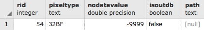
Now, to do something a bit more useful, run some basic statistic functions on this raster tile.
First, let's compute the summary statistics (count, mean, standard deviation, min, and max) with ST_SummaryStats() for an specific raster, in this case, number 54:
WITH stats AS (SELECT (ST_SummaryStats(rast, 1)).* FROM prism WHERE rid = 54) SELECT count, sum, round(mean::numeric, 2) AS mean, round(stddev::numeric, 2) AS stddev, min, max FROM stats;
The output of the preceding code will be as follows:
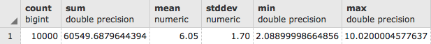
In the summary statistics, if the count indicates less than 10,000 (1002), it means that the raster is 10,000-count/100. In this case, the raster tile is about 0% NODATA.
Let's see how the values of the raster tile are distributed with ST_Histogram():
WITH hist AS ( SELECT (ST_Histogram(rast, 1)).* FROM chp05.prism WHERE rid = 54 ) SELECT round(min::numeric, 2) AS min, round(max::numeric, 2) AS max, count, round(percent::numeric, 2) AS percent FROM hist ORDER BY min;
The output will look as follows:
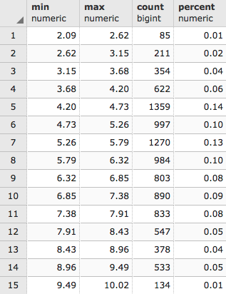
It looks like about 78% of all of the values are at or below 1370.50. Another way to see how the pixel values are distributed is to use ST_Quantile():
SELECT (ST_Quantile(rast, 1)).* FROM chp05.prism WHERE rid = 54;
The output of the preceding code is as follows:
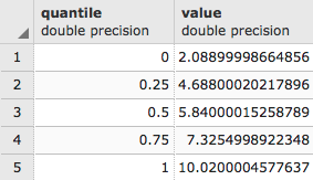
Let's see what the top 10 occurring values are in the raster tile with ST_ValueCount():
SELECT (ST_ValueCount(rast, 1)).* FROM chp05.prism WHERE rid = 54 ORDER BY count DESC, value LIMIT 10;
The output of the code is as follows:
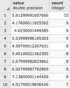
The ST_ValueCount allows other combinations of parameters that will allow rounding up of the values in order to aggregate some of the results, but a previous subset of values to look for must be defined; for example, the following code will count the appearance of values 2, 3, 2.5, 5.612999 and 4.176 rounded to the fifth decimal point 0.00001:
SELECT (ST_ValueCount(rast, 1, true, ARRAY[2,3,2.5,5.612999,4.176]::double precision[] ,0.0001)).* FROM chp05.prism WHERE rid = 54 ORDER BY count DESC, value LIMIT 10;
The results show the number of elements that appear similar to the rounded-up values in the array. The two values borrowed from the results on the previous figure, confirm the counting:
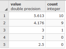
In the first part of this recipe, we looked at the metadata of the prism raster table and a single raster tile. We focused on that single raster tile to run a variety of statistics. The statistics provided some idea of what the data looks like.
We mentioned that the pixel values looked wrong when we looked at the output from ST_SummaryStats(). This same issue continued in the output from subsequent statistics functions. We also found that the values were in Celsius degrees. In the next recipe, we will recompute all the pixel values to their true values with a map-algebra operation.
In the previous recipe, we saw that the values in the PRISM rasters did not look correct for temperature values. After looking at the PRISM metadata, we learned that the values were scaled by 100.
In this recipe, we will process the scaled values to get the true values. Doing this will prevent future end-user confusion, which is always a good thing.
PostGIS provides two types of map-algebra functions, both of which return a new raster with one band. The type you use depends on the problem being solved and the number of raster bands involved.
The first map-algebra function (ST_MapAlgebra() or ST_MapAlgebraExpr()) depends on a valid, user-provided PostgreSQL algebraic expression that is called for every pixel. The expression can be as simple as an equation, or as complex as a logic-heavy SQL expression. If the map-algebra operation only requires at most two raster bands, and the expression is not complicated, you should have no problems using the expression-based map-algebra function.
The second map-algebra function (ST_MapAlgebra(), ST_MapAlgebraFct(), or ST_MapAlgebraFctNgb()) requires the user to provide an appropriate PostgreSQL function to be called for each pixel. The function being called can be written in any of the PostgreSQL PL languages (for example, PL/pgSQL, PL/R, PL/Perl), and be as complex as needed. This type is more challenging to use than the expression map-algebra function type, but it has the flexibility to work on any number of raster bands.
For this recipe, we use only the expression-based map-algebra function, ST_MapAlgebra(), to create a new band with the temperature values in Fahrenheit, and then append this band to the processed raster. If you are not using PostGIS 2.1 or a later version, use the equivalent ST_MapAlgebraExpr() function.
With any operation that is going to take a while and/or modify a stored raster, it is best to test that operation to ensure there are no mistakes and the output looks correct.
Let's run ST_MapAlgebra() on one raster tile, and compare the summary statistics before and after the map-algebra operation:
WITH stats AS (
SELECT
'before' AS state,
(ST_SummaryStats(rast, 1)).*
FROM chp05.prism
WHERE rid = 54
UNION ALL
SELECT
'after' AS state, (ST_SummaryStats(ST_MapAlgebra(rast, 1, '32BF', '([rast]*9/5)+32', -9999), 1 )).*
FROM chp05.prism
WHERE rid = 54
)
SELECT
state,
count,
round(sum::numeric, 2) AS sum,
round(mean::numeric, 2) AS mean,
round(stddev::numeric, 2) AS stddev,
round(min::numeric, 2) AS min,
round(max::numeric, 2) AS max
FROM stats ORDER BY state DESC;
The output looks as follows:
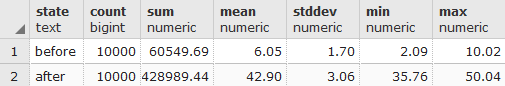
In the ST_MapAlgebra() function, we indicate that the output raster's band will have a pixel type of 32BF and a NODATA value of -9999. We use the expression '([rast]*9/5)+32' to convert each pixel value to its new value in Fahrenheit. Before ST_MapAlgebra() evaluates the expression, the pixel value replaces the placeholder '[rast]'. There are several other placeholders available, and they can be found in the ST_MapAlgebra() documentation.
Looking at the summary statistics and comparing the before and after processing, we see that the map-algebra operation works correctly. So, let's correct the entire table. We will append the band created from ST_MapAlgebra() to the existing raster:
UPDATE chp05.prism SET rast = ST_AddBand(rast, ST_MapAlgebra(rast, 1, '32BF', '([rast]*9/5)+32', -999), 1 ); ERROR: new row for relation "prism" violates check constraint " enforce_nodata_values_rast"
The SQL query will not work. Why? If you remember, when we loaded the PRISM rasters, we instructed raster2pgsql to add the standard constraints with the -C flag. It looks like we violated at least one of those constraints.
When installed, the standard constraints enforce a set of rules on each value of a raster column in the table. These rules guarantee that each raster column value has the same (or appropriate) attributes. The standard constraints comprise the following rules:
The error message indicates that we violated the out-db constraint. But we can't accept the error message as it is, because we are not doing anything related to out-db. All we are doing is adding a second band to the raster. Adding the second band violates the out-db constraint, because the constraint is prepared only for one band in the raster, not a raster with two bands.
We will have to drop the constraints, make our changes, and reapply the constraints:
SELECT DropRasterConstraints('chp05', 'prism', 'rast'::name);
After this command, we will have the following output showing the constraints were dropped:
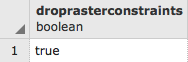
UPDATE chp05.prism SET rast = ST_AddBand(rast, ST_MapAlgebra(rast, 1, '32BF', ' ([rast]*9/5)+32', -9999), 1);
SELECT AddRasterConstraints('chp05', 'prism', 'rast'::name);
The UPDATE will take some time, and the output will look as follows, showing that the constraints were added again:
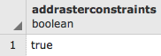
There is not much information provided in the output, so we will inspect the rasters. We will look at one raster tile:
SELECT (ST_Metadata(rast)).numbands FROM chp05.prism WHERE rid = 54;
The output is as follows:
The raster has two bands. The following are the details of these two bands:
SELECT 1 AS bandnum, (ST_BandMetadata(rast, 1)).* FROM chp05.prism WHERE rid = 54 UNION ALL SELECT 2 AS bandnum, (ST_BandMetadata(rast, 2)).* FROM chp05.prism WHERE rid = 54 ORDER BY bandnum;
The output looks as follows:
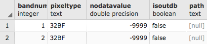
The first band is the same as the new second band with the correct attributes (the 32BF pixel type, and the NODATA value of -9999) that we specified in the call to ST_MapAlgebra().The real test, though, is to look at the summary statistics:
WITH stats AS (
SELECT
1 AS bandnum,
(ST_SummaryStats(rast, 1)).*
FROM chp05.prism
WHERE rid = 54
UNION ALL
SELECT
2 AS bandnum,
(ST_SummaryStats(rast, 2)).*
FROM chp05.prism
WHERE rid = 54
)
SELECT
bandnum,
count,
round(sum::numeric, 2) AS sum,
round(mean::numeric, 2) AS mean,
round(stddev::numeric, 2) AS stddev,
round(min::numeric, 2) AS min,
round(max::numeric, 2) AS max
FROM stats ORDER BY bandnum;
The output is as follows:
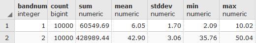
The summary statistics show that band 2 is correct after the values from band 1 were transformed into Fahrenheit; that is, the mean temperature is 6.05 of band 1 in degrees Celsius, and 42.90 in degrees Fahrenheit in band 2).
In this recipe, we applied a simple map-algebra operation with ST_MapAlgebra() to correct the pixel values. In a later recipe, we will present an advanced map-algebra operation to demonstrate the power of ST_MapAlgebra().
In the previous two recipes, we ran basic statistics only on one raster tile. Though running operations on a specific raster is great, it is not very helpful for answering real questions. In this recipe, we will use geometries to filter, clip, and unite raster tiles so that we can answer questions for a specific area.
We will use the San Francisco boundaries geometry previously imported into the sfpoly table. If you have not imported the boundaries, refer to the first recipe of this chapter for instructions.
Since we are to look at rasters in the context of San Francisco, an easy question to ask is: what was the average temperature for March, 2017 in San Francisco? Have a look at the following code:
SELECT (ST_SummaryStats(ST_Union(ST_Clip(prism.rast, 1, ST_Transform(sf.geom, 4269), TRUE)), 1)).mean FROM chp05.prism JOIN chp05.sfpoly sf ON ST_Intersects(prism.rast, ST_Transform(sf.geom, 4269)) WHERE prism.month_year = '2017-03-01'::date;
In the preceding SQL query, there are four items to pay attention to, which are as follows:
The following output shows the average minimum temperature for San Francisco:
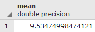
San Francisco was really cold in March, 2017. So, how does the rest of 2017 look? Is San Francisco always cold?
SELECT prism.month_year, (ST_SummaryStats(ST_Union(ST_Clip(prism.rast, 1, ST_Transform(sf.geom, 4269), TRUE)), 1)).mean FROM chp05.prism JOIN chp05.sfpoly sf ON ST_Intersects(prism.rast, ST_Transform(sf.geom, 4269)) GROUP BY prism.month_year ORDER BY prism.month_year;
The only change from the prior SQL query is the removal of the WHERE clause and the addition of a GROUP BY clause. Since ST_Union() is an aggregate function, we need to group the clipped rasters by month_year.
The output is as follows:
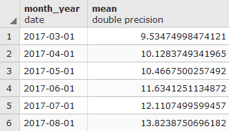
Based on the results, the late summer months of 2017 were the warmest, though not by a huge margin.
By using a geometry to filter the rasters in the prism table, only a small set of rasters needed clipping with the geometry and unionizing to compute the mean. This maximized the query performance, and more importantly, provided the answer to our question.
In the last recipe, we used the geometries to filter and clip rasters only to the areas of interest. The ST_Clip() and ST_Intersects() functions implicitly converted the geometry before relating it to the raster.
PostGIS provides several functions for converting rasters to geometries. Depending on the function, a pixel can be returned as an area or a point.
PostGIS provides one function for converting geometries to rasters.
In this recipe, we will convert rasters to geometries, and geometries to rasters. We will use the ST_DumpAsPolygons() and ST_PixelsAsPolygons() functions to convert rasters to geometries. We will then convert geometries to rasters using ST_AsRaster().
Let's adapt part of the query used in the last recipe to find out the average minimum temperature in San Francisco. We replace ST_SummaryStats() with ST_DumpAsPolygons(), and then return the geometries as WKT:
WITH geoms AS (SELECT ST_DumpAsPolygons(ST_Union(ST_Clip(prism.rast, 1, ST_Transform(sf.geom, 4269), TRUE)), 1 ) AS gv FROM chp05.prism
JOIN chp05.sfpoly sf ON ST_Intersects(prism.rast, ST_Transform(sf.geom, 4269)) WHERE prism.month_year = '2017-03-01'::date ) SELECT (gv).val, ST_AsText((gv).geom) AS geom FROM geoms;
The output is as follows:
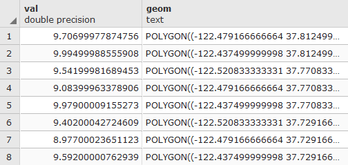
Now, replace the ST_DumpAsPolygons() function with ST_PixelsAsPolyons():
WITH geoms AS (SELECT (ST_PixelAsPolygons(ST_Union(ST_Clip(prism.rast, 1, ST_Transform(sf.geom, 4269), TRUE)), 1 )) AS gv FROM chp05.prism JOIN chp05.sfpoly sf ON ST_Intersects(prism.rast, ST_Transform(sf.geom, 4269)) WHERE prism.month_year = '2017-03-01'::date) SELECT (gv).val, ST_AsText((gv).geom) AS geom FROM geoms;
The output is as follows:
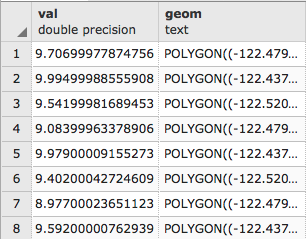
Again, the query results have been trimmed. What is important is the number of rows returned. ST_PixelsAsPolygons() returns significantly more geometries than ST_DumpAsPolygons(). This is due to the different mechanism used in each function.
The following images show the difference between ST_DumpAsPolygons() and ST_PixelsAsPolygons(). The ST_DumpAsPolygons() function only dumps pixels with a value and unites these pixels with the same value. The ST_PixelsAsPolygons() function does not merge pixels and dumps all of them, as shown in the following diagrams:
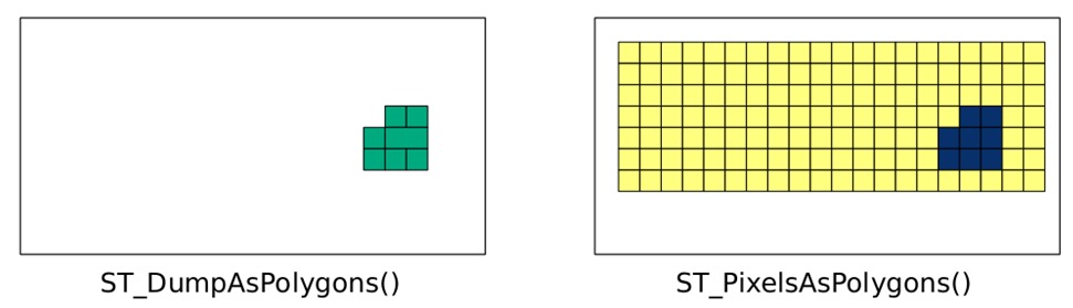
The ST_PixelsAsPolygons() function returns one geometry for each pixel. If there are 100 pixels, there will be 100 geometries. Each geometry of ST_DumpAsPolygons() is the union of all of the pixels in an area with the same value. If there are 100 pixels, there may be up to 100 geometries.
There is one other significant difference between ST_PixelAsPolygons() and ST_DumpAsPolygons(). Unlike ST_DumpAsPolygons(), ST_PixelAsPolygons() returns a geometry for pixels with the NODATA value, and has an empty value for the val column.
Let's convert a geometry to a raster with ST_AsRaster(). We insert ST_AsRaster() to return a raster with a pixel size of 100 by -100 meters containing four bands of the pixel type 8BUI. Each of these bands will have a pixel NODATA value of 0, and a specific pixel value (29, 194, 178, and 255 for each band respectively). The units for the pixel size are determined by the geometry's projection, which is also the projection of the created raster:
SELECT ST_AsRaster( sf.geom, 100., -100., ARRAY['8BUI', '8BUI', '8BUI', '8BUI']::text[], ARRAY[29, 194, 178, 255]::double precision[], ARRAY[0, 0, 0, 0]::double precision[] ) FROM sfpoly sf;
If we visualize the generated raster of San Francisco's boundaries and overlay the source geometry, we get the following result, which is a zoomed-in view of the San Francisco boundary's geometry converted to a raster with ST_AsRaster():
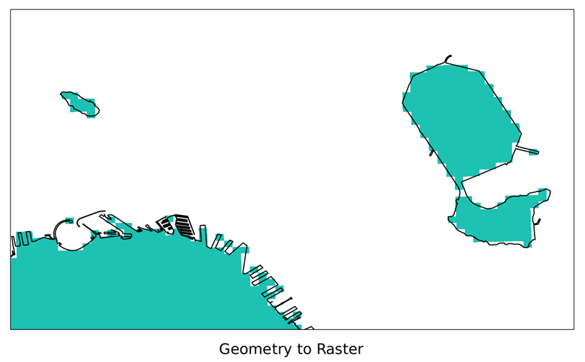
Though it is great that the geometry is now a raster, relating the generated raster to other rasters requires additional processing. This is because the generated raster and the other raster will most likely not be aligned. If the two rasters are not aligned, most PostGIS raster functions do not work. The following figure shows two non-aligned rasters (simplified to pixel grids):
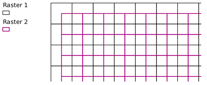
When a geometry needs to be converted to a raster so as to relate to an existing raster, use that existing raster as a reference when calling ST_AsRaster():
SELECT ST_AsRaster( sf.geom, prism.rast, ARRAY['8BUI', '8BUI', '8BUI', '8BUI']::text[], ARRAY[29, 194, 178, 255]::double precision[], ARRAY[0, 0, 0, 0]::double precision[] ) FROM chp05.sfpoly sf CROSS JOIN chp05.prism WHERE prism.rid = 1;
In the preceding query, we use the raster tile at rid = 1 as our reference raster. The ST_AsRaster() function uses the reference raster's metadata to create the geometry's raster. If the geometry and reference raster have different SRIDs, the geometry is transformed to the same SRID before creating the raster.
In this recipe, we converted rasters to geometries. We also created new rasters from geometries. The ability to convert between rasters and geometries allows the use of functions that would otherwise not be possible.
Though PostGIS has plenty of functions for working with rasters, it is sometimes more convenient and more efficient to work on the source rasters before importing them into the database. One of the times when working with rasters outside the database is more efficient is when the raster contains subdatasets, typically found in HDF4, HDF5, and NetCDF files.
In this recipe, we will preprocess a MODIS raster with the GDAL VRT format to filter and rearrange the subdatasets. Internally, a VRT file is comprised of XML tags. This means we can create a VRT file with any text editor. But since creating a VRT file manually can be tedious, we will use the gdalbuildvrt utility.
The MODIS raster we use is provided by NASA, and is available in the source package.
You will need GDAL built with HDF4 support to continue with this recipe, as MODIS rasters are usually in the HDF4-EOS format.
The following screenshot shows the MODIS raster used in this recipe and the next two recipes. In the following image, we see parts of California, Nevada, Arizona, and Baja California:
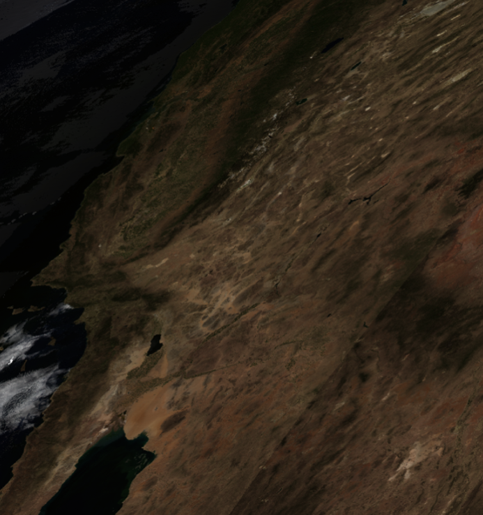
To allow PostGIS to properly support MODIS rasters, we will also need to add the MODIS Sinusoidal projection to the spatial_ref_sys table.
On the command line, navigate to the MODIS directory:
> cd C:\postgis_cookbook\data\chap05\MODIS
In the MODIS directory, there should be several files. One of these files has the name srs.sql and contains the INSERT statement needed for the MODIS Sinusoidal projection. Run the INSERT statement:
> psql -d postgis_cookbook -f srs.sql
The main file has the extension HDF. Let's check the metadata of that HDF file:
> gdalinfo MYD09A1.A2012161.h08v05.005.2012170065756.hdf
When run, gdalinfo outputs a lot of information. We are looking for the list of subdatasets found in the Subdatasets section:
Subdatasets:
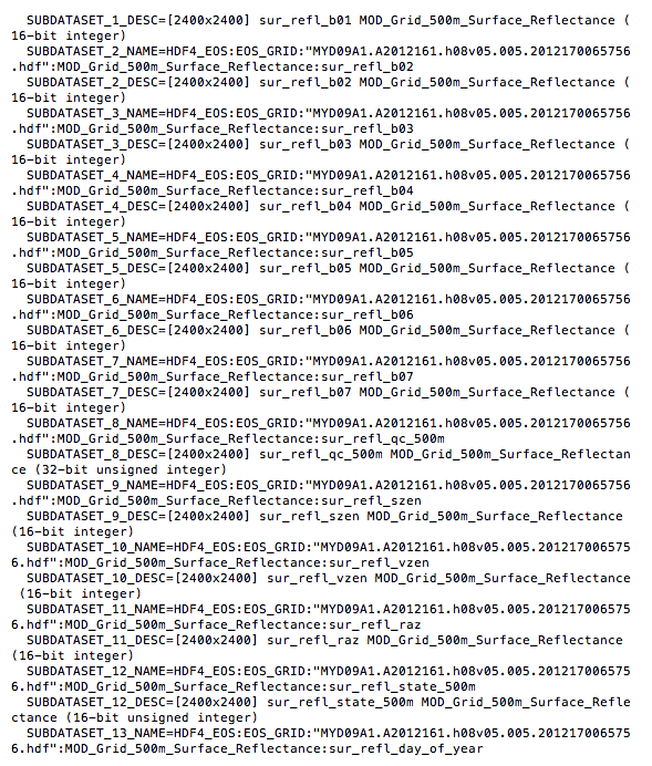
Each subdataset is one variable of the MODIS raster included in the source code for this chapter. For our purposes, we only need the first four subdatasets, which are as follows:
The VRT format allows us to select the subdatasets to be included in the VRT raster as well as change the order of the subdatasets. We want to rearrange the subdatasets so that they are in the RGB order.
Let's call gdalbuildvrt to create a VRT file for our MODIS raster. Do not run the following!
> gdalbuildvrt -separate modis.vrt
HDF4_EOS:EOS_GRID:"MYD09A1.A2012161.h08v05.005.2012170065756.hdf":MOD_Grid_500m_Surface_Reflectance:sur_refl_b01
HDF4_EOS:EOS_GRID:"MYD09A1.A2012161.h08v05.005.2012170065756.hdf":MOD_Grid_500m_Surface_Reflectance:sur_refl_b04
HDF4_EOS:EOS_GRID:"MYD09A1.A2012161.h08v05.005.2012170065756.hdf":MOD_Grid_500m_Surface_Reflectance:sur_refl_b03
HDF4_EOS:EOS_GRID:"MYD09A1.A2012161.h08v05.005.2012170065756.hdf":MOD_Grid_500m_Surface_Reflectance:sur_refl_b02
We really hope you did not run the preceding code. The command does work but is too long and cumbersome. It would be better if we can pass a file indicating the subdatasets to include and their order in the VRT. Thankfully, gdalbuildvrt provides such an option with the -input_file_list flag.
In the MODIS directory, the modis.txt file can be passed to gdalbuildvrt with the -input_file_list flag. Each line of the modis.txt file is the name of a subdataset. The order of the subdatasets in the text file dictates the placement of each subdataset in the VRT:
HDF4_EOS:EOS_GRID:"MYD09A1.A2012161.h08v05.005.2012170065756.hdf":MOD_Grid_500m_Surface_Reflectance:sur_refl_b01 HDF4_EOS:EOS_GRID:"MYD09A1.A2012161.h08v05.005.2012170065756.hdf":MOD_Grid_500m_Surface_Reflectance:sur_refl_b04 HDF4_EOS:EOS_GRID:"MYD09A1.A2012161.h08v05.005.2012170065756.hdf":MOD_Grid_500m_Surface_Reflectance:sur_refl_b03 HDF4_EOS:EOS_GRID:"MYD09A1.A2012161.h08v05.005.2012170065756.hdf":MOD_Grid_500m_Surface_Reflectance:sur_refl_b02
Now, call gdalbuildvrt with modis.txt in the following manner:
> gdalbuildvrt -separate -input_file_list modis.txt modis.vrt
Feel free to inspect the generated modis.vrt VRT file in your favorite text editor. Since the contents of the VRT file are just XML tags, it is easy to make additions, changes, and deletions.
We will do one last thing before importing our processed MODIS raster into PostGIS. We will convert the VRT file to a GeoTIFF file with the gdal_translate utility, because not all applications have built-in support for HDF4, HDF5, NetCDF, or VRT, and the superior portability of GeoTIFF:
> gdal_translate -of GTiff modis.vrt modis.tif
Finally, import modis.tif with raster2pgsql:
> raster2pgsql -s 96974 -F -I -C -Y modis.tif chp05.modis | psql -d postgis_cookbook
The raster2pgsql supports a long list of input formats. You can call the command with the option -G to see the complete list.
This recipe was all about processing a MODIS raster into a form suitable for use in PostGIS. We used the gdalbuildvrt utility to create our VRT. As a bonus, we used gdal_translate to convert between raster formats; in this case, from VRT to GeoTIFF.
If you're feeling particularly adventurous, try using gdalbuildvrt to create a VRT of the 12 PRISM rasters with each raster as a separate band.
In the previous recipe, we processed a MODIS raster to extract only those subdatasets that are of interest, in a more suitable order. Once done with the extraction, we imported the MODIS raster into its own table.
Here, we make use of the warping capabilities provided in PostGIS. This ranges from simply transforming the MODIS raster to a more suitable projection, to creating an overview by resampling the pixel size.
We will use several PostGIS warping functions, specifically ST_Transform() and ST_Rescale(). The ST_Transform() function reprojects a raster to a new spatial reference system (for example, from WGS84 to NAD83). The ST_Rescale() function shrinks or grows the pixel size of a raster.
The first thing we will do is transform our raster, since the MODIS rasters have their own unique spatial-reference system. We will convert the raster from MODIS Sinusoidal projection to US National Atlas Equal Area (SRID 2163).
Before we transform the raster, we will clip the MODIS raster with our San Francisco boundaries geometry. By clipping our raster before transformation, the operation takes less time than it does to transform and then clip the raster:
SELECT ST_Transform(ST_Clip(m.rast, ST_Transform(sf.geom, 96974)), 2163) FROM chp05.modis m CROSS JOIN chp05.sfpoly sf;
The following image shows the clipped MODIS raster with the San Francisco boundaries on top for comparison:
When we call ST_Transform() on the MODIS raster, we only pass the destination SRID 2163. We could specify other parameters, such as the resampling algorithm and error tolerance. The default resampling algorithm and error tolerance are set to NearestNeighbor and 0.125. Using a different algorithm and/or lowering the error tolerance may improve the quality of the resampled raster at the cost of more processing time.
Let's transform the MODIS raster again, this time specifying the resampling algorithm and error tolerance as Cubic and 0.05, respectively. We also indicate that the transformed raster must be aligned to a reference raster:
SELECT ST_Transform(ST_Clip(m.rast, ST_Transform(sf.geom, 96974)),
prism.rast, 'cubic', 0.05) FROM chp05.modis m CROSS JOIN chp05.prism CROSS JOIN chp05.sfpoly sf WHERE prism.rid = 1;
Unlike the prior queries where we transform the MODIS raster, let's create an overview. An overview is a lower-resolution version of the source raster. If you are familiar with pyramids, an overview is level one of a pyramid, while the source raster is the base level:
WITH meta AS (SELECT (ST_Metadata(rast)).* FROM chp05.modis) SELECT ST_Rescale(modis.rast, meta.scalex * 4., meta.scaley * 4., 'cubic') AS rast FROM chp05.modis CROSS JOIN meta;
The overview is 25% of the resolution of the original MODIS raster. This means four times the scale, and one quarter the width and height. To prevent hardcoding the desired scale X and scale Y, we use the MODIS raster's scale X and scale Y returned by ST_Metadata(). As you can see in the following image, the overview has a coarser resolution:
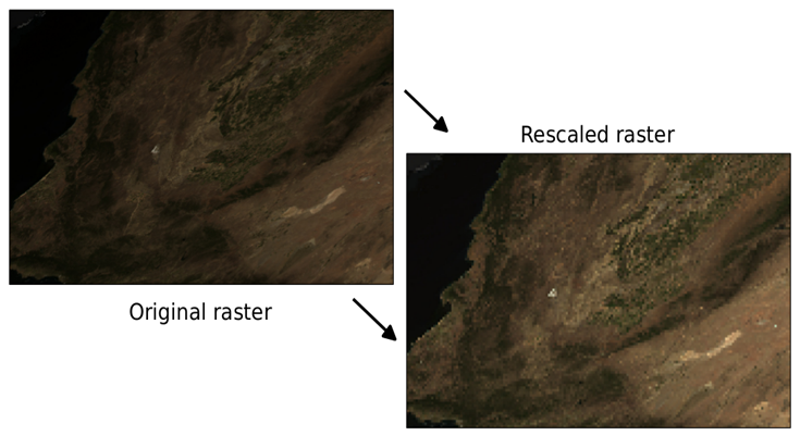
Using some of PostGIS's resampling capabilities, we projected the MODIS raster to a different spatial reference with ST_Transform() as well as controlled the quality of the projected raster. We also created an overview with ST_Rescale().
Using these functions and other PostGIS resampling functions, you should be able to manipulate all the rasters.
In a prior recipe, we used the expression-based map-algebra function ST_MapAlgebra() to convert the PRISM pixel values to their true values. The expression-based ST_MapAlgebra() method is easy to use, but limited to operating on at most two raster bands. This restricts the ST_MapAlgebra() function's usefulness for processes that require more than two input raster bands, such as the Normalized Difference Vegetation Index (NDVI) and the Enhanced Vegetation Index (EVI).
There is a variant of ST_MapAlgebra() designed to support an unlimited number of input raster bands. Instead of taking an expression, this ST_MapAlgebra() variant requires a callback function. This callback function is run for each set of input pixel values, and returns either a new pixel value, or NULL for the output pixel. Additionally, this variant of ST_MapAlgebra() permits operations on neighborhoods (sets of pixels around a center pixel).
PostGIS comes with a set of ready-to-use ST_MapAlgebra() callback functions. All of these functions are intended for neighborhood calculations, such as computing the average value of a neighborhood, or interpolating empty pixel values.
We will use the MODIS raster to compute the EVI. EVI is a three-band operation consisting of the red, blue, and near-infrared bands. To do an ST_MapAlgebra() operation on three bands, PostGIS 2.1 or a higher version is required.
To use ST_MapAlgebra() on more than two bands, we must use the callback function variant. This means we need to create a callback function. Callback functions can be written in any PostgreSQL PL language, such as PL/pgSQL or PL/R. Our callback functions are all written in PL/pgSQL, as this language is always included with a base PostgreSQL installation.
Our callback function uses the following equation to compute the three-band EVI:

The following code implements the MODIS EVI function in SQL:
CREATE OR REPLACE FUNCTION chp05.modis_evi(value double precision[][][], "position" int[][], VARIADIC userargs text[])
RETURNS double precision
AS $$
DECLARE
L double precision;
C1 double precision;
C2 double precision;
G double precision;
_value double precision[3];
_n double precision;
_d double precision;
BEGIN
-- userargs provides coefficients
L := userargs[1]::double precision;
C1 := userargs[2]::double precision;
C2 := userargs[3]::double precision;
G := userargs[4]::double precision;
-- rescale values, optional
_value[1] := value[1][1][1] * 0.0001;
_value[2] := value[2][1][1] * 0.0001;
_value[3] := value[3][1][1] * 0.0001;
-- value can't be NULL
IF
_value[1] IS NULL OR
_value[2] IS NULL OR
_value[3] IS NULL
THEN
RETURN NULL;
END IF;
-- compute numerator and denominator
_n := (_value[3] - _value[1]);
_d := (_value[3] + (C1 * _value[1]) - (C2 * _value[2]) + L);
-- prevent division by zero
IF _d::numeric(16, 10) = 0.::numeric(16, 10) THEN
RETURN NULL;
END IF;
RETURN G * (_n / _d);
END;
$$ LANGUAGE plpgsql IMMUTABLE;
If you can't create the function, you probably do not have the necessary privileges in the database.
There are several characteristics required for all of the callback functions. These are as follows:
value = ARRAY[ 1 =>
[ -- raster 1 [pixval, pixval, pixval], -- row of raster 1 [pixval, pixval, pixval], [pixval, pixval, pixval] ], 2 => [ -- raster 2 [pixval, pixval, pixval], -- row of raster 2 [pixval, pixval, pixval], [pixval, pixval, pixval] ], ... N => [ -- raster N [pixval, pixval, pixval], -- row of raster [pixval, pixval, pixval], [pixval, pixval, pixval] ] ]; pos := ARRAY[ 0 => [x-coordinate, y-coordinate], -- center pixel o f output raster 1 => [x-coordinate, y-coordinate], -- center pixel o f raster 1 2 => [x-coordinate, y-coordinate], -- center pixel o f raster 2 ... N => [x-coordinate, y-coordinate], -- center pixel o f raster N ]; userargs := ARRAY[ 'arg1', 'arg2', ... 'argN' ];
If the callback functions are not correctly structured, the ST_MapAlgebra() function will fail or behave incorrectly.
In the function body, we convert the user arguments to their correct datatypes, rescale the pixel values, check that no pixel values are NULL (arithmetic operations with NULL values always result in NULL), compute the numerator and denominator components of EVI, check that the denominator is not zero (prevent division by zero), and then finish the computation of EVI.
Now we call our callback function, modis_evi(), with ST_MapAlgebra():
SELECT ST_MapAlgebra(rast, ARRAY[1, 3, 4]::int[], -- only use the red, blue a nd near infrared bands 'chp05.modis_evi(
double precision[], int[], text[])'::regprocedure,
-- signature for callback function '32BF',
-- output pixel type 'FIRST', NULL, 0, 0, '1.', -- L '6.', -- C1 '7.5', -- C2 '2.5' -- G ) AS rast FROM modis m;
In our call to ST_MapAlgebra(), there are three criteria to take note of, which are as follows:
The following images show the MODIS raster before and after running the EVI operation. The EVI raster has a pale white to dark green colormap applied for highlighting areas of high vegetation:
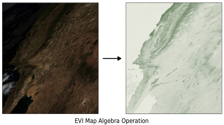
For the two-band EVI, we will use the following callback function. The two-band EVI equation is computed with the following code:
CREATE OR REPLACE FUNCTION chp05.modis_evi2(value1 double precision, value2 double precision, pos int[], VARIADIC userargs text[])
RETURNS double precision
AS $$
DECLARE
L double precision;
C double precision;
G double precision;
_value1 double precision;
_value2 double precision;
_n double precision;
_d double precision;
BEGIN
-- userargs provides coefficients
L := userargs[1]::double precision;
C := userargs[2]::double precision;
G := userargs[3]::double precision;
-- value can't be NULL
IF
value1 IS NULL OR
value2 IS NULL
THEN
RETURN NULL;
END IF;
_value1 := value1 * 0.0001;
_value2 := value2 * 0.0001;
-- compute numerator and denominator
_n := (_value2 - _value1);
_d := (L + _value2 + (C * _value1));
-- prevent division by zero
IF _d::numeric(16, 10) = 0.::numeric(16, 10) THEN
RETURN NULL;
END IF;
RETURN G * (_n / _d);
END;
$$ LANGUAGE plpgsql IMMUTABLE;
Like ST_MapAlgebra() callback functions, ST_MapAlgebraFct() requires callback functions to be structured in a specific manner. There is a difference between the callback function for ST_MapAlgebraFct() and the prior one for ST_MapAlgebra(). This function has two simple pixel-value parameters instead of an array for all pixel values:
SELECT ST_MapAlgebraFct( rast, 1, -- red band rast, 4, -- NIR band 'modis_evi2(double precision, double precision, int[], text[])'::regprocedure,
-- signature for callback function '32BF', -- output pixel type 'FIRST', '1.', -- L '2.4', -- C '2.5' -- G) AS rast FROM chp05.modis m;
Besides the difference in function names, ST_MapAlgebraFct() is called differently than ST_MapAlgebra(). The same raster is passed to ST_MapAlgebraFct() twice. The other difference is that there is one less user-defined argument being passed to the callback function, as the two-band EVI has one less coefficient.
We demonstrated some of the advanced uses of PostGIS's map-algebra functions by computing the three-band and two-band EVIs from our MODIS raster. This was achieved using ST_MapAlgebra() and ST_MapAlgebraFct(), respectively. With some planning, PostGIS's map-algebra functions can be applied to other uses, such as edge detection and contrast stretching.
For additional practice, write your own callback function to generate an NDVI raster from the MODIS raster. The equation for NDVI is: NDVI = ((IR - R)/(IR + R)) where IR is the pixel value on the infrared band, and R is the pixel value on the red band. This index generates values between -1.0 and 1.0, in which negative values usually represent non-green elements (water, snow, clouds), and values close to zero represent rocks and deserted land.
PostGIS comes with several functions for use on digital elevation model (DEM) rasters to solve terrain-related problems. Though these problems have historically been in the hydrology domain, they can now be found elsewhere; for example, finding the most fuel-efficient route from point A to point B or determining the best location on a roof for a solar panel. PostGIS 2.0 introduced ST_Slope(), ST_Aspect(), and ST_HillShade() while PostGIS 2.1 added the new functions ST_TRI(), ST_TPI(), and ST_Roughness(), and new variants of existing elevation functions.
We will use the SRTM raster, loaded as 100 x 100 tiles, in this chapter's first recipe. With it, we will generate slope and hillshade rasters using San Francisco as our area of interest.
The next two queries in the How to do it section use variants of ST_Slope() and ST_HillShade() that are only available in PostGIS 2.1 or higher versions. The new variants permit the specification of a custom extent to constrain the processing area of the input raster.
Let's generate a slope raster from a subset of our SRTM raster tiles using ST_Slope(). A slope raster computes the rate of elevation change from one pixel to a neighboring pixel:
WITH r AS ( -- union of filtered tiles
SELECT ST_Transform(ST_Union(srtm.rast), 3310) AS rast
FROM chp05.srtm
JOIN chp05.sfpoly sf ON ST_DWithin(ST_Transform(srtm.rast::geometry,
3310), ST_Transform(sf.geom, 3310), 1000)),
cx AS ( -- custom extent
SELECT ST_AsRaster(ST_Transform(sf.geom, 3310), r.rast) AS rast
FROM chp05.sfpoly sf CROSS JOIN r
)
SELECT ST_Clip(ST_Slope(r.rast, 1, cx.rast), ST_Transform(sf.geom, 3310)) AS rast FROM r
CROSS JOIN cx
CROSS JOIN chp05.sfpoly sf;
All spatial objects in this query are projected to California Albers (SRID 3310), a projection with units in meters. This projection eases the use of ST_DWithin() to broaden our area of interest to include the tiles within 1,000 meters of San Francisco's boundaries, which improves the computed slope values for the pixels at the edges of the San Francisco boundaries. We also use a rasterized version of our San Francisco boundaries as the custom extent for restricting the computed area. After running ST_Slope(), we clip the slope raster just to San Francisco.
We can reuse the ST_Slope() query and substitute ST_HillShade() for ST_Slope() to create a hillshade raster, showing how the sun would illuminate the terrain of the SRTM raster:
WITH r AS ( -- union of filtered tiles
SELECT ST_Transform(ST_Union(srtm.rast), 3310) AS rast
FROM chp05.srtm
JOIN chp05.sfpoly sf ON ST_DWithin(ST_Transform(srtm.rast::geometry,
3310), ST_Transform(sf.geom, 3310), 1000)),
cx AS ( -- custom extent
SELECT ST_AsRaster(ST_Transform(sf.geom, 3310), r.rast) AS rast FROM chp05.sfpoly sf CROSS JOIN r)
SELECT ST_Clip(ST_HillShade(r.rast, 1, cx.rast),ST_Transform(sf.geom, 3310)) AS rast FROM r
CROSS JOIN cx
CROSS JOIN chp05.sfpoly sf;
In this case, ST_HillShade() is a drop-in replacement for ST_Slope() because we do not specify any special input parameters for either function. If we need to specify additional arguments for ST_Slope() or ST_HillShade(), all changes are confined to just one line.
The following images show the SRTM raster before and after processing it with ST_Slope() and ST_HillShade():
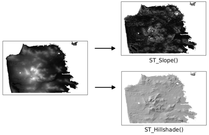
As you can see in the screenshot, the slope and hillshade rasters help us better understand the terrain of San Francisco.
If PostGIS 2.0 is available, we can still use 2.0's ST_Slope() and ST_HillShade() to create slope and hillshade rasters. But there are several differences you need to be aware of, which are as follows:
We can adapt our ST_Slope() query from the beginning of this recipe by removing the creation and application of the custom extent. Since the custom extent constrained the computation to just a specific area, the inability to specify such a constraint means PostGIS 2.0's ST_Slope() will perform slower:
WITH r AS ( -- union of filtered tiles SELECT ST_Transform(ST_Union(srtm.rast), 3310) AS rast FROM srtm JOIN sfpoly sf ON ST_DWithin(ST_Transform(srtm.rast::geometry, 3310),
ST_Transform(sf.geom, 3310), 1000) ) SELECT ST_Clip(ST_Slope(r.rast, 1), ST_Transform(sf.geom, 3310)) AS rast FROM r CROSS JOIN sfpoly sf;
The DEM functions in PostGIS allowed us to quickly analyze our SRTM raster. In the basic use cases, we were able to swap one function for another without any issues.
What is impressive about these DEM functions is that they are all wrappers around ST_MapAlgebra(). The power of ST_MapAlgebra() is in its adaptability to different problems.
In Chapter 4, Working with Vector Data – Advanced Recipes, we used gdal_translate to export PostGIS rasters to a file. This provides a method for transferring files from one user to another, or from one location to another. The only problem with this method is that you may not have access to the gdal_translate utility.
A different but equally functional approach is to use the ST_AsGDALRaster() family of functions available in PostGIS. In addition to ST_AsGDALRaster(), PostGIS provides ST_AsTIFF(), ST_AsPNG(), and ST_AsJPEG() to support the most common raster file formats.
To easily visualize raster files without the need for a GIS application, PostGIS 2.1 and later versions provide ST_ColorMap(). This function applies a built-in or user-specified color palette to a raster, that upon exporting with ST_AsGDALRaster(), can be viewed with any image viewer, such as a web browser.
In this recipe, we will use ST_AsTIFF() and ST_AsPNG()to export rasters to GeoTIFF and PNG file formats, respectively. We will also apply the ST_ColorMap() so that we can see them in any image viewer.
To enable GDAL drivers in PostGIS, you should run the following command in pgAdmin:
SET postgis.gdal_enabled_drivers = 'ENABLE_ALL'; SELECT short_name FROM ST_GDALDrivers();
The following queries can be run in a standard SQL client, such as psql or pgAdminIII; however, we can't use the returned output because the output has escaped, and these clients do not undo the escaping. Applications with lower-level API functions can unescape the query output. Examples of this would be a PHP script, a pass-a-record element to pg_unescape_bytea(), or a Python script using Psycopg2's implicit decoding while fetching a record. A sample PHP script (save_raster_to_file.php) can be found in this chapter's data directory.
Let us say that a colleague asks for the monthly minimum temperature data for San Francisco during the summer months as a single raster file. This entails restricting our PRISM rasters to June, July, and August, clipping each monthly raster to San Francisco's boundaries, creating one raster with each monthly raster as a band, and then outputting the combined raster to a portable raster format. We will convert the combined raster to the GeoTIFF format:
WITH months AS ( -- extract monthly rasters clipped to San Francisco SELECT prism.month_year, ST_Union(ST_Clip(prism.rast, 2, ST_Transform(sf.geom, 4269), TRUE)) AS rast FROM chp05.prism JOIN chp05.sfpoly sf ON ST_Intersects(prism.rast, ST_Transform(sf.geom, 4269)) WHERE prism.month_year BETWEEN '2017-06-01'::date AND '2017-08-01'::date GROUP BY prism.month_year ORDER BY prism.month_year ), summer AS ( -- new raster with each monthly raster as a band SELECT ST_AddBand(NULL::raster, array_agg(rast)) AS rast FROM months) SELECT -- export as GeoTIFF ST_AsTIFF(rast) AS content FROM summer;
To filter our PRISM rasters, we use ST_Intersects() to keep only those raster tiles that spatially intersect San Francisco's boundaries. We also remove all rasters whose relevant month is not June, July, or August. We then use ST_AddBand() to create a new raster with each summer month's new raster band. Finally, we pass the combined raster to ST_AsTIFF() to generate a GeoTIFF.
If you output the returned value from ST_AsTIFF() to a file, run gdalinfo on that file. The gdalinfo output shows that the GeoTIFF file has three bands, and the coordinate system of SRID 4322:
Driver: GTiff/GeoTIFF
Files: surface.tif
Size is 20, 7
Coordinate System is:
GEOGCS["WGS 72",
DATUM["WGS_1972",
SPHEROID["WGS 72",6378135,298.2600000000045, AUTHORITY["EPSG","7043"]],
TOWGS84[0,0,4.5,0,0,0.554,0.2263], AUTHORITY["EPSG","6322"]],
PRIMEM["Greenwich",0], UNIT["degree",0.0174532925199433],
AUTHORITY["EPSG","4322"]]
Origin = (-123.145833333333314,37.937500000000114)
Pixel Size = (0.041666666666667,-0.041666666666667)
Metadata:
AREA_OR_POINT=Area
Image Structure Metadata:
INTERLEAVE=PIXEL
Corner Coordinates:
Upper Left (-123.1458333, 37.9375000) (123d 8'45.00"W, 37d56'15.00"N)
Lower Left (-123.1458333, 37.6458333) (123d 8'45.00"W, 37d38'45.00"N)
Upper Right (-122.3125000, 37.9375000) (122d18'45.00"W, 37d56'15.00"N)
Lower Right (-122.3125000, 37.6458333) (122d18'45.00"W, 37d38'45.00"N)
Center (-122.7291667, 37.7916667) (122d43'45.00"W, 37d47'30.00"N)
Band 1 Block=20x7 Type=Float32, ColorInterp=Gray
NoData Value=-9999
Band 2 Block=20x7 Type=Float32, ColorInterp=Undefined
NoData Value=-9999
Band 3 Block=20x7 Type=Float32, ColorInterp=Undefined
NoData Value=-9999
The problem with the GeoTIFF raster is that we generally can't view it in a standard image viewer. If we use ST_AsPNG() or ST_AsJPEG(), the image generated is much more readily viewable. But PNG and JPEG images are limited by the supported pixel types 8BUI and 16BUI (PNG only). Both formats are also limited to, at the most, three bands (four, if there is an alpha band).
To help get around various file format limitations, we can use ST_MapAlgebra(), ST_Reclass() , or ST_ColorMap(), for this recipe. The ST_ColorMap() function converts a raster band of any pixel type to a set of up to four 8BUI bands. This facilitates creating a grayscale, RGB, or RGBA image that is then passed to ST_AsPNG(), or ST_AsJPEG().
Taking our query for computing a slope raster of San Francisco from our SRTM raster in a prior recipe, we can apply one of ST_ColorMap() function's built-in colormaps, and then pass the resulting raster to ST_AsPNG() to create a PNG image:
WITH r AS (SELECT ST_Transform(ST_Union(srtm.rast), 3310) AS rast FROM chp05.srtm JOIN chp05.sfpoly sf ON ST_DWithin(ST_Transform(srtm.rast::geometry, 3310),
ST_Transform(sf.geom, 3310), 1000) ), cx AS ( SELECT ST_AsRaster(ST_Transform(sf.geom, 3310), r.rast) AS rast FROM sfpoly sf CROSS JOIN r ) SELECT ST_AsPNG(ST_ColorMap(ST_Clip(ST_Slope(r.rast, 1, cx.rast), ST_Transform(sf.geom, 3310) ), 'bluered')) AS rast FROM r CROSS JOIN cx CROSS JOIN chp05.sfpoly sf;
The bluered colormap sets the minimum, median, and maximum pixel values to dark blue, pale white, and bright red, respectively. Pixel values between the minimum, median, and maximum values are assigned colors that are linearly interpolated from the minimum to median or median to maximum range. The resulting image readily shows where the steepest slopes in San Francisco are.
The following is a PNG image generated by applying the bluered colormap with ST_ColorMap() and ST_AsPNG(). The pixels in red represent the steepest slopes:
In our use of ST_AsTIFF() and ST_AsPNG(), we passed the raster to be converted as the sole argument. Both of these functions have additional parameters to customize the output TIFF or PNG file. These additional parameters include various compression and data organization settings.
Using ST_AsTIFF() and ST_AsPNG(), we exported rasters from PostGIS to GeoTIFF and PNG. The ST_ColorMap() function helped generate images that can be opened in any image viewer. If we needed to export these images to a different format supported by GDAL, we would use ST_AsGDALRaster().
In this chapter, we will cover the following topics:
So far, we have used PostGIS as a vector and raster tool, using relatively simple relationships between objects and simple structures. In this chapter, we review an additional PostGIS-related extension: pgRouting. pgRouting allows us to interrogate graph structures in order to answer questions such as "What is the shortest route from where I am to where I am going?" This is an area that is heavily occupied by the existing web APIs (such as Google, Bing, MapQuest, and others) and services, but it can be better served by rolling our own services for many use cases. Which cases? It might be a good idea to create our own services in situations where we are trying to answer questions that aren't answered by the existing services; where the data available to us is better or more applicable; or where we need or want to avoid the terms of service conditions for these APIs.
pgRouting is a separate extension used in addition to PostGIS, which is now available in the PostGIS bundle on the Application Stack Builder (recommended for Windows). It can also be downloaded and installed by DEB, RPM, and macOS X packages and Windows binaries available at http://pgrouting.org/download.html.
For macOS users, it is recommended that you use the source packages available on Git (https://github.com/pgRouting/pgrouting/releases), and use CMake, available at https://cmake.org/download/, to make the installation build.
Packages for Linux Ubuntu users can be found at http://trac.osgeo.org/postgis/wiki/UsersWikiPostGIS22UbuntuPGSQL95Apt.
pgRouting doesn't deal well with nondefault schemas, so before we begin, we will set the schema in our user preferences using the following command:
ALTER ROLE me SET search_path TO chp06,public;
Next, we need to add the pgrouting extension to our database. If PostGIS is not already installed on the database, we'll need to add it as an extension as well:
CREATE EXTENSION postgis; CREATE EXTENSION pgrouting;
We will start by loading a test dataset. You can get some really basic sample data from http://docs.pgrouting.org/latest/en/sampledata.html.
This sample data consists of a small grid of streets in which any functions can be run.
Then, run the create table and data insert scripts available at the dataset website. You should make adjustments to preserve the schema structure for chp06—for example:
CREATE TABLE chp06.edge_table (
id BIGSERIAL,
dir character varying,
source BIGINT,
target BIGINT,
cost FLOAT,
reverse_cost FLOAT,
capacity BIGINT,
reverse_capacity BIGINT,
category_id INTEGER,
reverse_category_id INTEGER,
x1 FLOAT,
y1 FLOAT,
x2 FLOAT,
y2 FLOAT,
the_geom geometry
);
Now that the data is loaded, let's build topology on the table (if you haven't already done this during the data-load process):
SELECT pgr_createTopology('chp06.edge_table',0.001);
Building a topology creates a new node table—chp06.edge_table_vertices_pgr—for us to view. This table will aid us in developing queries.
Now that the data is loaded, we can run a quick test. We'll use a simple algorithm called Dijkstra to calculate the shortest path from node 5 to node 12.
An important point to note is that the nodes created in pgRouting during the topology creation process are created unintentionally for some versions. This has been patched in future versions, but for some versions of pgRouting, this means that your node numbers will not be the same as those we use here in the book. View your data in an application to determine which nodes to use or whether you should use a k-nearest neighbors search for the node nearest to a static geographic point. See Chapter 11, Using Desktop Clients, for more information on viewing PostGIS data and Chapter 4, Working with Vector Data – Advanced Recipes, for approaches to finding the nearest node automatically:
SELECT * FROM pgr_dijkstra( 'SELECT id, source, target, cost FROM chp06.edge_table_vertices_pgr', 2, 9, );
The preceding query will result in the following:
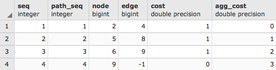
When we ask for a route using Dijkstra and other routing algorithms, the result often comes in the following form:
For example, to get the geometry back, we need to rejoin the edge IDs with the original table. To make this approach work transparently, we will use the WITH common table expression to create a temporary table to which we will join our geometry:
WITH dijkstra AS (
SELECT pgr_dijkstra(
'SELECT id, source, target, cost, x1, x2, y1, y2
FROM chp06.edge_table', 2, 9
)
)
SELECT id, ST_AsText(the_geom)
FROM chp06.edge_table et, dijkstra d
WHERE et.id = (d.pgr_dijkstra).edge;
The preceding code will give the following output:
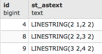
Congratulations! You have just completed a route in pgRouting. The following diagram illustrates this scenario:
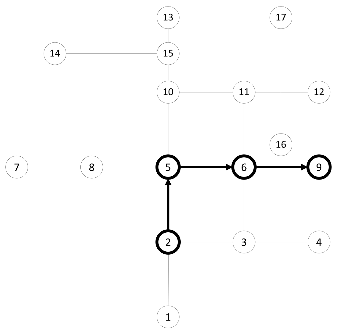
Test data is great for understanding how algorithms work, but the real data is often more interesting. A good source for real data worldwide is OpenStreetMap (OSM), a worldwide, accessible, wiki-style, geospatial dataset. What is wonderful about using OSM in conjunction with pgRouting is that it is inherently a topological model, meaning that it follows the same kinds of rules in its construction as we do in graph traversal within pgRouting. Because of the way editing and community participation works in OSM, it is often an equally good or better data source than commercial ones and is, of course, quite compatible with our open source model.
Another great feature is that there is free and open source software to ingest OSM data and import it into a routing database—osm2pgrouting.
It is recommended that you get the downloadable files from the example dataset that we have provided, available at http://www.packtpub.com/support. You will be using the XML OSM data. You can also get custom extracts directly from the web interface at http://www.openstreetmap.org/or by using the overpass turbo interface to access OSM data (https://overpass-turbo.eu/), but this could limit the area we would be able to extract.
Once we have the data, we need to unzip it using our favorite compression utility. Double-clicking on the file to unzip it will typically work on Windows and macOS machines. Two good utilities for unzipping on Linux are bunzip2 and zip. What will remain is an XML extract of the data we want for routing. In our use case, we are downloading the data for the greater Cleveland area.
Now we need a utility for placing this data into a routable database. An example of one such tool is osm2pgrouting, which can be downloaded and compiled using the instructions at http://github.com/pgRouting/osm2pgrouting. Use CMake from https://cmake.org/download/ to make the installation build in macOS. For Linux Ubuntu users there is an available package at https://packages.ubuntu.com/artful/osm2pgrouting.
When osm2pgrouting is run without anything set, the output shows us the options that are required and available to use with osm2pgrouting:
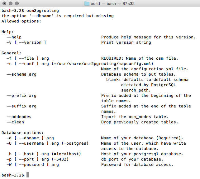
To run the osm2pgrouting command, we have a small number of required parameters. Double-check the paths pointing to mapconfig.xml and cleveland.osm before running the following command:
osm2pgrouting --file cleveland.osm --conf /usr/share/osm2pgrouting/mapconfig.xml --dbname postgis_cookbook --user me --schema chp06 --host localhost --prefix cleveland_ --clean
Our dataset may be quite large, and could take some time to process and import—be patient. The end of the output should say something like the following:
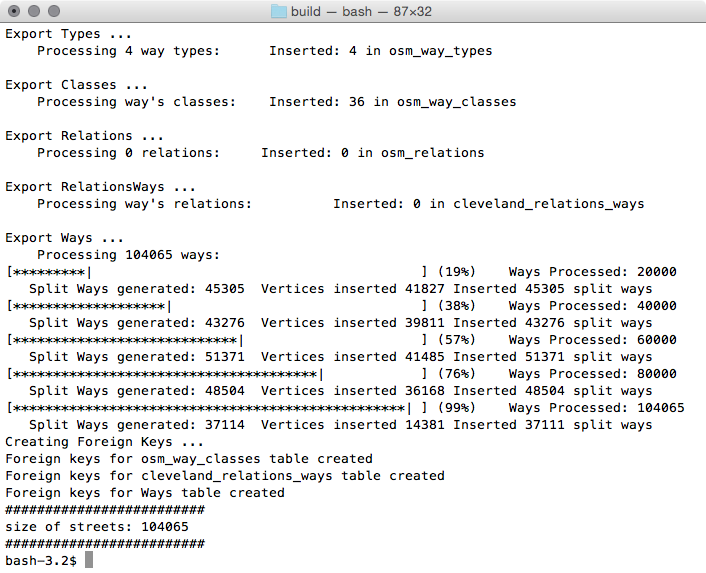
Our new vector table, by default, is named cleveland_ways. If no -prefix flag was used, the table name would just be ways.
You should have the created following tables:
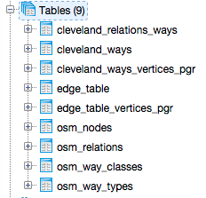
osm2pgrouting is a powerful tool that handles a lot of the translation of OSM data into a format that can be used in pgRouting. In this case, it creates eight tables from our input file. Of those eight, we'll address the two primary tables: the ways table and the nodes table.
Our ways table is a table of the lines that represent all our streets, roads, and trails that are in OSM. The nodes table contains all the intersections. This helps us identify the beginning and end points for routing.
Let's apply an A* ("A star") routing approach to this problem.
You will recognize the following syntax from Dijkstra:
WITH astar AS (
SELECT * FROM pgr_astar(
'SELECT gid AS id, source, target,
length AS cost, x1, y1, x2, y2
FROM chp06.cleveland_ways', 89475, 14584, false
)
)
SELECT gid, the_geom
FROM chp06.cleveland_ways w, astar a
WHERE w.gid = a.edge;
The following screenshot shows the results displayed on a map (map tiles by Stamen Design, under CC BY 3.0; data by OpenStreetMap, under CC BY SA):
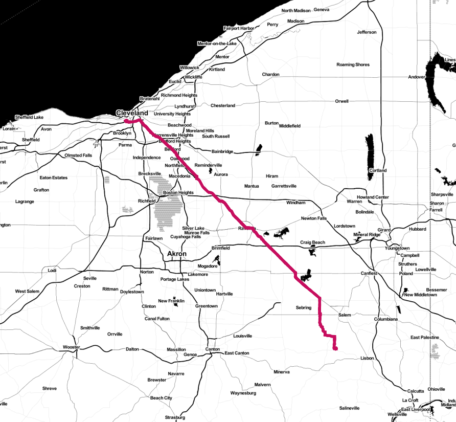
Driving distance (pgr_drivingDistance) is a query that calculates all nodes within the specified driving distance of a starting node. This is an optional function compiled with pgRouting; so if you compile pgRouting yourself, make sure that you enable it and include the CGAL library, an optional dependency for pgr_drivingDistance.
Driving distance is useful when user sheds are needed that give realistic driving distance estimates, for example, for all customers with five miles driving, biking, or walking distance. These estimates can be contrasted with buffering techniques, which assume no barrier to travelling and are useful for revealing the underlying structures of our transportation networks relative to individual locations.
We will load the same dataset that we used in the Startup – Dijkstra routing recipe. Refer to this recipe to import data.
In the following example, we will look at all users within a distance of three units from our starting point—that is, a proposed bike shop at node 2:
SELECT * FROM pgr_drivingDistance(
'SELECT id, source, target, cost FROM chp06.edge_table',
2, 3
);
The preceding command gives the following output:
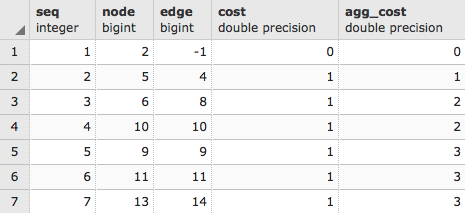
As usual, we just get a list from the pgr_drivingDistance table that, in this case, comprises sequence, node, edge cost, and aggregate cost. PgRouting, like PostGIS, gives us low-level functionality; we need to reconstruct what geometries we need from that low-level functionality. We can use that node ID to extract the geometries of all of our nodes by executing the following script:
WITH DD AS (
SELECT * FROM pgr_drivingDistance(
'SELECT id, source, target, cost
FROM chp06.edge_table', 2, 3
)
)
SELECT ST_AsText(the_geom)
FROM chp06.edge_table_vertices_pgr w, DD d
WHERE w.id = d.node;
The preceding command gives the following output:
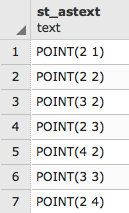
But the output seen is just a cluster of points. Normally, when we think of driving distance, we visualize a polygon. Fortunately, we have the pgr_alphaShape function that provides us that functionality. This function expects id, x, and y values for input, so we will first change our previous query to convert to x and y from the geometries in edge_table_vertices_pgr:
WITH DD AS (
SELECT * FROM pgr_drivingDistance(
'SELECT id, source, target, cost FROM chp06.edge_table',
2, 3
)
)
SELECT id::integer, ST_X(the_geom)::float AS x, ST_Y(the_geom)::float AS y
FROM chp06.edge_table_vertices_pgr w, DD d
WHERE w.id = d.node;
The output is as follows:
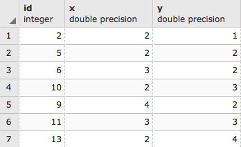
Now we can wrap the preceding script up in the alphashape function:
WITH alphashape AS (
SELECT pgr_alphaShape('
WITH DD AS (
SELECT * FROM pgr_drivingDistance(
''SELECT id, source, target, cost
FROM chp06.edge_table'', 2, 3
)
),
dd_points AS(
SELECT id::integer, ST_X(the_geom)::float AS x,
ST_Y(the_geom)::float AS y
FROM chp06.edge_table_vertices_pgr w, DD d
WHERE w.id = d.node
)
SELECT * FROM dd_points
')
),
So first, we will get our cluster of points. As we did earlier, we will explicitly convert the text to geometric points:
alphapoints AS ( SELECT ST_MakePoint((pgr_alphashape).x, (pgr_alphashape).y) FROM alphashape ),
Now that we have points, we can create a line by connecting them:
alphaline AS ( SELECT ST_Makeline(ST_MakePoint) FROM alphapoints ) SELECT ST_MakePolygon(ST_AddPoint(ST_Makeline, ST_StartPoint(ST_Makeline))) FROM alphaline;
Finally, we construct the line as a polygon using ST_MakePolygon. This requires adding the start point by executing ST_StartPoint in order to properly close the polygon. The complete code is as follows:
WITH alphashape AS (
SELECT pgr_alphaShape('
WITH DD AS (
SELECT * FROM pgr_drivingDistance(
''SELECT id, source, target, cost
FROM chp06.edge_table'', 2, 3
)
),
dd_points AS(
SELECT id::integer, ST_X(the_geom)::float AS x,
ST_Y(the_geom)::float AS y
FROM chp06.edge_table_vertices_pgr w, DD d
WHERE w.id = d.node
)
SELECT * FROM dd_points
')
),
alphapoints AS (
SELECT ST_MakePoint((pgr_alphashape).x,
(pgr_alphashape).y)
FROM alphashape
),
alphaline AS (
SELECT ST_Makeline(ST_MakePoint) FROM alphapoints
)
SELECT ST_MakePolygon(
ST_AddPoint(ST_Makeline, ST_StartPoint(ST_Makeline))
)
FROM alphaline;
Our first driving distance calculation can be better understood in the context of the following diagram, where we can reach nodes 9, 11, 13 from node 2 with a driving distance of 3:
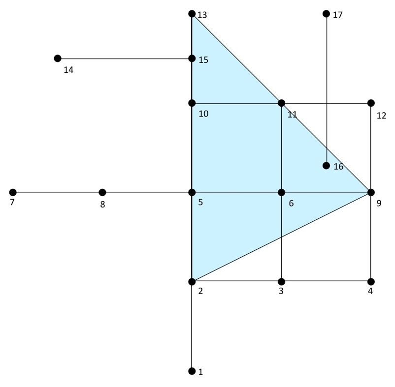
In the Using polygon overlays for proportional census estimates recipe in Chapter 2, Structures That Work, we employed a simple buffer around a trail alignment in conjunction with the census data to get estimates of what the demographics were of the people within walking distance of the trail, estimated as a mile long. The problem with this approach, of course, is that it assumes that it is an "as the crow flies" estimate. In reality, rivers, large roads, and roadless stretches serve as real barriers to people's movement through space. Using pgRouting's pgr_drivingDistance function, we can realistically simulate people's movement on the routable networks and get better estimates. For our use case, we'll keep the simulation a bit simpler than a trail alignment—we'll consider the demographics of a park facility, say, the Cleveland Metroparks Zoo, and potential bike users within 4 miles of it, which adds up approximately to a 15-minute bike ride.
For our analysis, we will use the proportional_sum function from Chapter 2, Structures That Work, so if you have not added this to your PostGIS tool belt, run the following commands:
CREATE OR REPLACE FUNCTION chp02.proportional_sum(geometry, geometry, numeric) RETURNS numeric AS $BODY$ SELECT $3 * areacalc FROM ( SELECT (ST_Area(ST_Intersection($1, $2))/ST_Area($2))::numeric AS areacalc ) AS areac ; $BODY$ LANGUAGE sql VOLATILE;
The proportional_sum function will take our input geometry into account and the count value of the population and return an estimate of the proportional population.
Now we need to load our census data. Use the following command:
shp2pgsql -s 3734 -d -i -I -W LATIN1 -g the_geom census chp06.census | psql -U me -d postgis_cookbook -h localhost
Also, if you have not yet loaded the data mentioned in the Loading data from OpenStreetMap and finding the shortest path A* recipe, take the time to do so now.
Once all the data is entered, we can proceed with the analysis.
The pgr_drivingdistance polygon we created is the first step in the demographic analysis. Refer to the Driving distance/service area calculation recipe if you need to familiarize yourself with its use. In this case, we'll consider the cycling distance. The nearest node to the Cleveland Metroparks Zoo is 24746, according to our loaded dataset; so we'll use that as the center point for our pgr_drivingdistance calculation and we'll use approximately 6 kilometers as our distance, as we want to know the number of zoo visitors within this distance of the Cleveland Metroparks Zoo. However, since our data is using 4326 EPSG, the distance we will give the function will be in degrees, so 0.05 will give us an approximate distance of 6 km that will work with the pgr_drivingDistance function:
CREATE TABLE chp06.zoo_bikezone AS (
WITH alphashape AS (
SELECT pgr_alphaShape('
WITH DD AS (
SELECT * FROM pgr_drivingDistance(
''SELECT gid AS id, source, target, reverse_cost
AS cost FROM chp06.cleveland_ways'',
24746, 0.05, false
)
),
dd_points AS(
SELECT id::int4, ST_X(the_geom)::float8 as x,
ST_Y(the_geom)::float8 AS y
FROM chp06.cleveland_ways_vertices_pgr w, DD d
WHERE w.id = d.node
)
SELECT * FROM dd_points
')
),
alphapoints AS (
SELECT ST_MakePoint((pgr_alphashape).x, (pgr_alphashape).y)
FROM alphashape
),
alphaline AS (
SELECT ST_Makeline(ST_MakePoint) FROM alphapoints
)
SELECT 1 as id, ST_SetSRID(ST_MakePolygon(ST_AddPoint(ST_Makeline, ST_StartPoint(ST_Makeline))), 4326) AS the_geom FROM alphaline
);
The preceding script gives us a very interesting shape (map tiles by Stamen Design, under CC BY 3.0; data by OpenStreetMap, under CC BY SA). See the following screenshot:
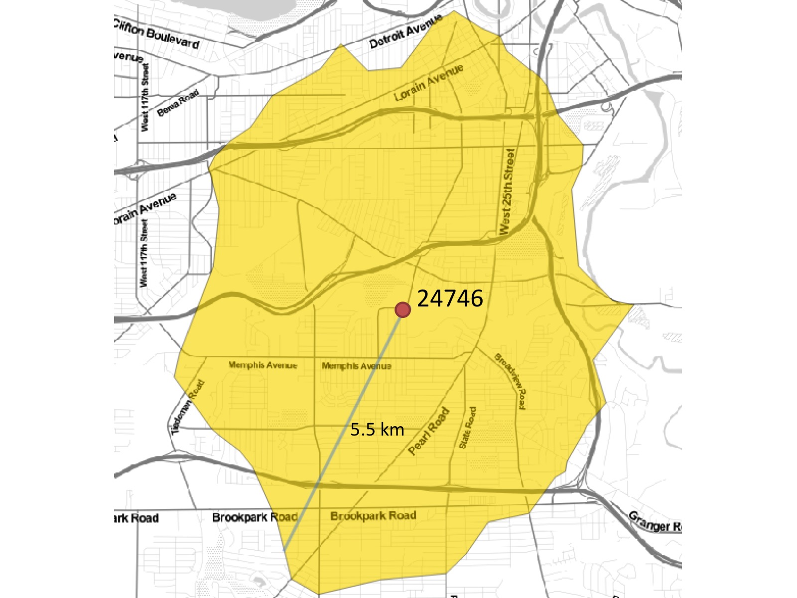
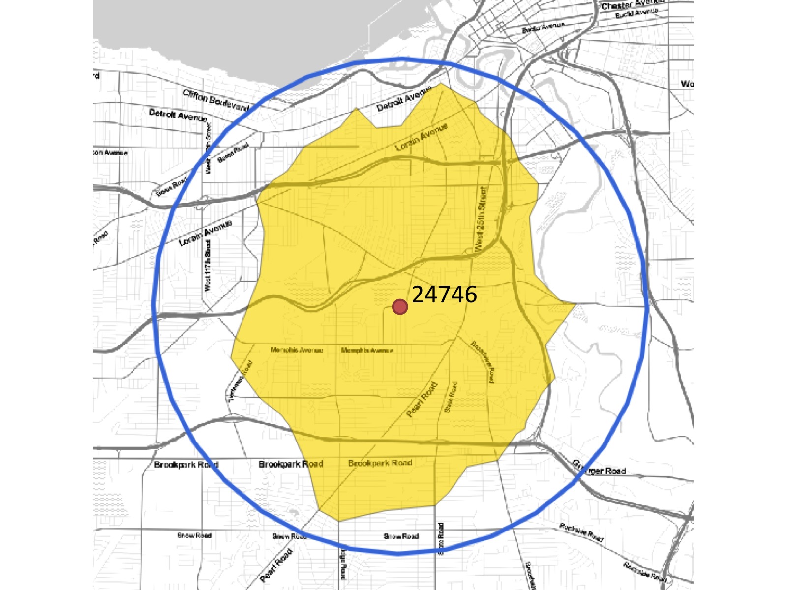
In the previous screenshot, we can see the difference between the cycling distance across the real road network, shaded in blue, and the equivalent 4-mile buffer or as-the-crow-flies distance. Let's apply this to our demographic analysis using the following script:
SELECT ROUND(SUM(chp02.proportional_sum(
ST_Transform(a.the_geom,3734), b.the_geom, b.pop))) AS population
FROM Chp06.zoo_bikezone AS a, chp06.census as b WHERE ST_Intersects(ST_Transform(a.the_geom, 3734), b.the_geom) GROUP BY a.id;
The output is as follows:
(1 row)
So, how does the preceding output compare to what we would get if we look at the buffered distance?
SELECT ROUND(SUM(chp02.proportional_sum(
ST_Transform(a.the_geom,3734), b.the_geom, b.pop))) AS population FROM (SELECT 1 AS id, ST_Buffer(ST_Transform(the_geom, 3734), 17000)
AS the_geom FROM chp06.cleveland_ways_vertices_pgr WHERE id = 24746 ) AS a, chp06.census as b WHERE ST_Intersects(ST_Transform(a.the_geom, 3734), b.the_geom) GROUP BY a.id;
(1 row)
The preceding output shows a difference of more than 60,000 people. In other words, using a buffer overestimates the population compared to using pgr_drivingdistance.
In several recipes in Chapter 4, Working with Vector Data – Advanced Recipes, we explored extracting Voronoi polygons from sets of points. In this recipe, we'll use the Voronoi function employed in the Using external scripts to embed new functionality to calculate Voronoi polygons section to serve as the first step in extracting the centerline of a polygon. One could also use the Using external scripts to embed new functionality to calculate Voronoi polygons—advanced recipe, which would run faster on large datasets. For this recipe, we will use the simpler but slower approach.
One additional dependency is that we will be using the chp02.polygon_to_line(geometry) function from the Normalizing internal overlays recipe in Chapter 2, Structures That Work.
What do we mean by the centerline of a polygon? Imagine a digitized stream flowing between its pair of banks, as shown in the following screenshot:
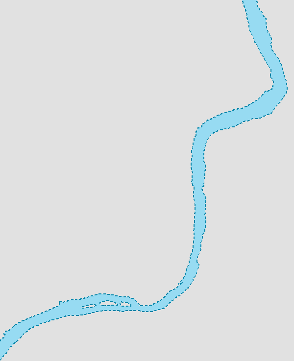
If we wanted to find the center of this in order to model the water flow, we could extract it using a skeletonization approach, as shown in the following screenshot:
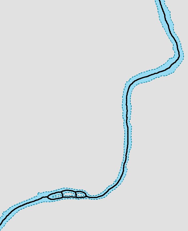
The difficulty with skeletonization approaches, as we'll soon see, is that they are often subject to noise, which is something that natural features such as our stream make plenty of. This means that typical skeletonization, which could be done simply with a Voronoi approach, is therefore inherently inadequate for our purposes.
This brings us to the reason why skeletonization is included in this chapter. Routing is a way for us to simplify skeletons derived from the Voronoi method. It allows us to trace from one end of a major feature to the other and skip all the noise in between.
As we will be using the Voronoi calculations from the Calculating Voronoi Diagram recipe in Chapter 4, Working with Vector Data – Advanced Recipes, you should refer to that recipe to prepare yourself for the functions used in this recipe.
We will use a stream dataset found in this book's source package under the hydrology folder. To load it, use the following command:
shp2pgsql -s 3734 -d -i -I -W LATIN1 -g the_geom ebrr_polygon chp06.voronoi_hydro | psql -U me -d postgis_cookbook
The streams we create will look as shown in the following screenshot:
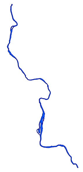
In order to perform the basic skeletonization, we'll calculate the Voronoi polygons on the nodes that make up the original stream polygon. By default, the edges of the Voronoi polygons find the line that demarcates the midpoint between points. We will leverage this tendency by treating our lines like points—adding extra points to the lines and then converting the lines to a point set. This approach, in combination with the Voronoi approach, will provide an initial estimate of the polygon's centerline.
We will add extra points to our input geometries using the ST_Segmentize function and then convert the geometries to points using ST_DumpPoints:
CREATE TABLE chp06.voronoi_points AS( SELECT (ST_DumpPoints(ST_Segmentize(the_geom, 5))).geom AS the_geom
FROM chp06.voronoi_hydro UNION ALL SELECT (ST_DumpPoints(ST_Extent(the_geom))).geom AS the_geom
FROM chp06.voronoi_hydro )
The following screenshot shows our polygons as a set of points if we view it on a desktop GIS:
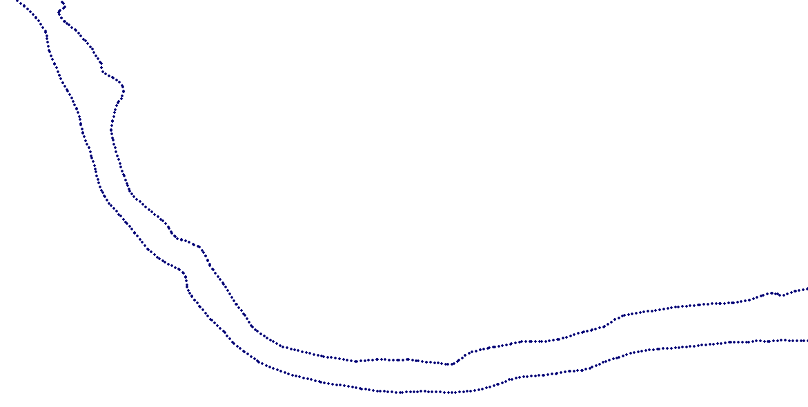
The set of points in the preceding screenshot is what we feed into our Voronoi calculation:
CREATE TABLE chp06.voronoi AS(
SELECT (ST_Dump(
ST_SetSRID(
ST_VoronoiPolygons(points.the_geom),
3734))).geom as the_geom
FROM (SELECT ST_Collect(ST_SetSRID(the_geom, 3734)) as the_geom FROM chp06.voronoi_points) as points);
The following screenshot shows a Voronoi diagram derived from our points:
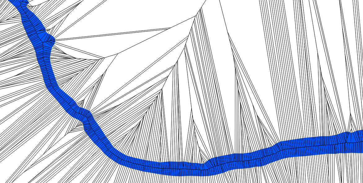
If you look closely at the preceding screenshot, you will see the basic centerline displayed in our new data. Now we will take the first step toward extracting it. We should index our inputs and then intersect the Voronoi output with the original stream polygon in order to clean the data back to something reasonable. In the extraction process, we'll also extract the edges from the polygons and remove the edges along the original polygon in order to remove any excess lines before our routing step. This is implemented in the following script:
CREATE INDEX chp06_voronoi_geom_gist
ON chp06.voronoi
USING gist(the_geom);
DROP TABLE IF EXISTS voronoi_intersect;
CREATE TABLE chp06.voronoi_intersect AS WITH vintersect AS (
SELECT ST_Intersection(ST_SetSRID(ST_MakeValid(a.the_geom), 3734),
ST_MakeValid(b.the_geom)) AS the_geom
FROM Chp06.voronoi a, chp06.voronoi_hydro b
WHERE ST_Intersects(ST_SetSRID(a.the_geom, 3734), b.the_geom)
),
linework AS (
SELECT chp02.polygon_to_line(the_geom) AS the_geom
FROM vintersect
),
polylines AS (
SELECT ((ST_Dump(ST_Union(lw.the_geom))).geom)
::geometry(linestring, 3734) AS the_geom
FROM linework AS lw
),
externalbounds AS (
SELECT chp02.polygon_to_line(the_geom) AS the_geom
FROM voronoi_hydro
)
SELECT (ST_Dump(ST_Union(p.the_geom))).geom
FROM polylines p, externalbounds b
WHERE NOT ST_DWithin(p.the_geom, b.the_geom, 5);
Now we have a second-level approximatio of the skeleton (shown in the following screenshot). It is messy, but it starts to highlight the centerline that we seek:
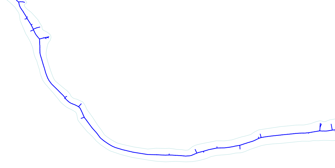
Now we are nearly ready for routing. The centerline calculation we have is a good approximation of a straight skeleton, but is still subject to the noisiness of the natural world. We'd like to eliminate that noisiness by choosing our features and emphasizing them through routing. First, we need to prepare the table to allow for routing calculations, as shown in the following commands:
ALTER TABLE chp06.voronoi_intersect ADD COLUMN gid serial;
ALTER TABLE chp06.voronoi_intersect ADD PRIMARY KEY (gid);
ALTER TABLE chp06.voronoi_intersect ADD COLUMN source integer;
ALTER TABLE chp06.voronoi_intersect ADD COLUMN target integer;
Then, to create a routable network from our skeleton, enter the following commands:
SELECT pgr_createTopology('voronoi_intersect', 0.001, 'the_geom', 'gid', 'source', 'target', 'true');
CREATE INDEX source_idx ON chp06.voronoi_intersect("source");
CREATE INDEX target_idx ON chp06.voronoi_intersect("target");
ALTER TABLE chp06.voronoi_intersect ADD COLUMN length double precision;
UPDATE chp06.voronoi_intersect SET length = ST_Length(the_geom);
ALTER TABLE chp06.voronoi_intersect ADD COLUMN reverse_cost double precision;
UPDATE chp06.voronoi_intersect SET reverse_cost = length;
Now we can route along the primary centerline of our polygon using the following commands:
CREATE TABLE chp06.voronoi_route AS
WITH dijkstra AS (
SELECT * FROM pgr_dijkstra('SELECT gid AS id, source, target, length
AS cost FROM chp06.voronoi_intersect', 10851, 3, false)
)
SELECT gid, geom
FROM voronoi_intersect et, dijkstra d
WHERE et.gid = d.edge;
If we look at the detail of this routing, we see the following:
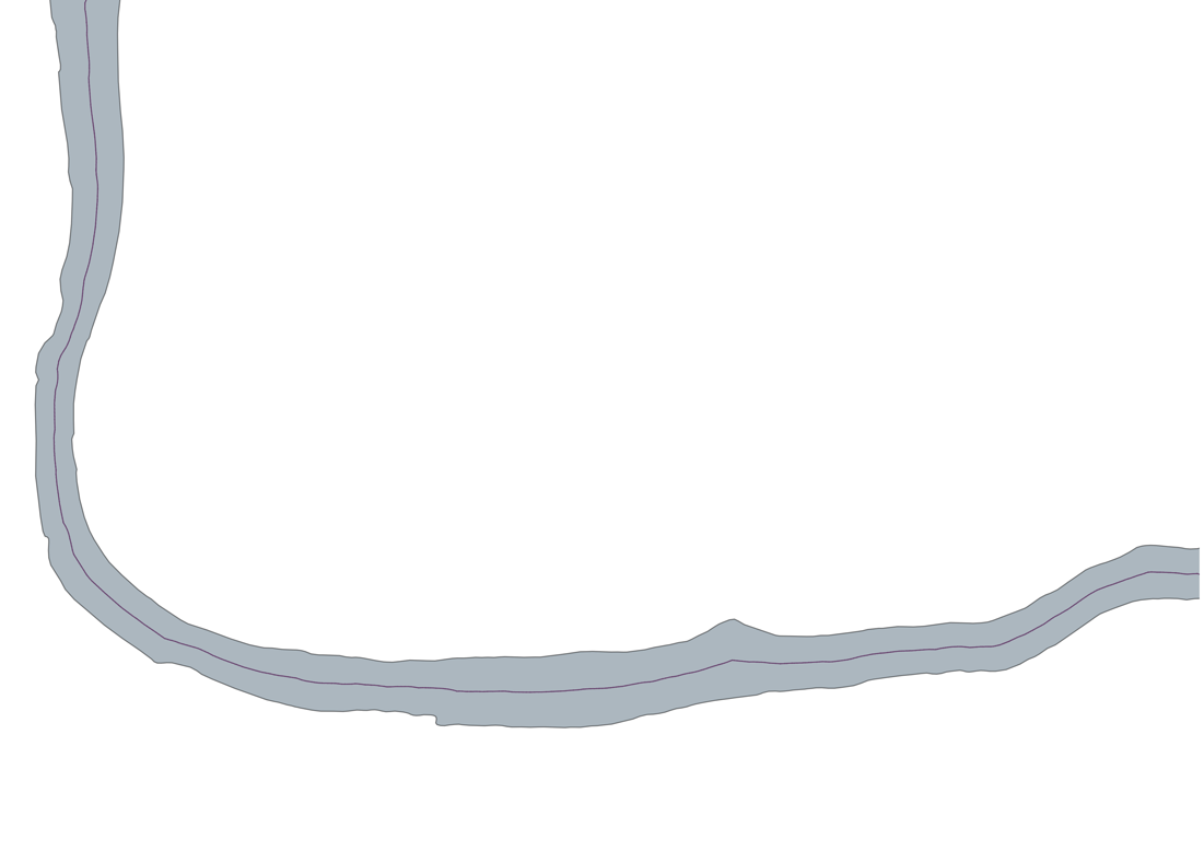
Now we can compare the original polygon with the trace of its centerline:
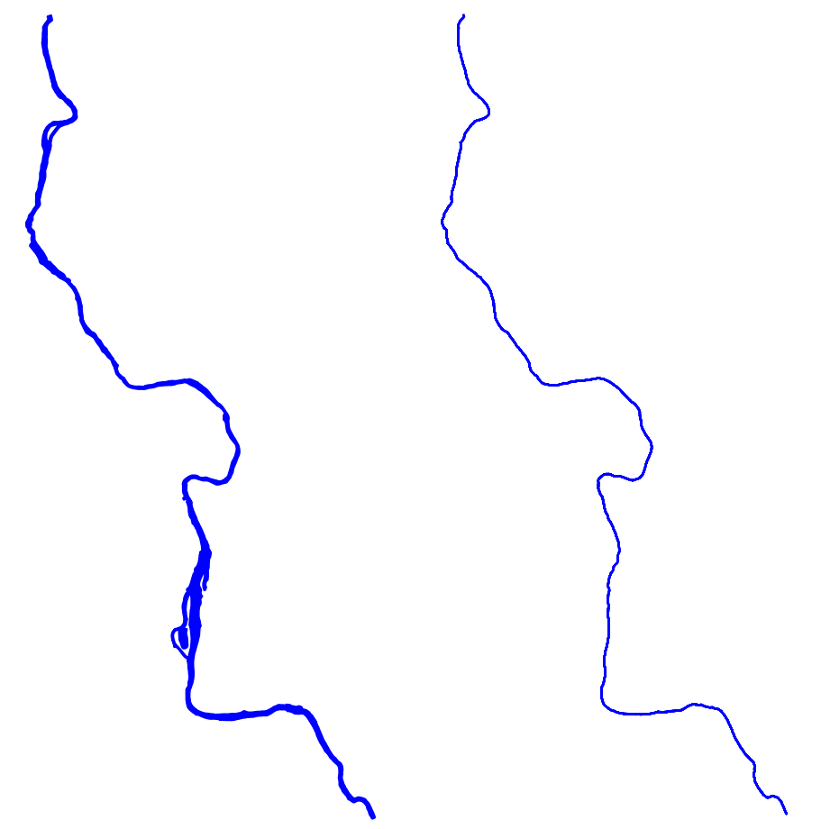
The preceding screenshot shows the original geometry of the stream in contrast to our centerline or skeleton. It is an excellent output that vastly simplifies our input geometry while retaining its relevant features.
In this chapter, we will cover:
In this chapter, we will explore the 3D capabilities of PostGIS. We will focus on three main categories: how to insert 3D data into PostGIS, how to analyze and perform queries using 3D data, and how to dump 3D data out of PostGIS. This chapter will use 3D point clouds as 3D data, including LiDAR data and those derived from Structure from Motion (SfM) techniques. Additionally, we will build a function that extrudes building footprints to 3D.
It is important to note that for this chapter, we will address the postgreSQL-pointcloud extension; point clouds are usually large data sets of a three dimensional representation of point coordinates in a coordinate system. Point clouds are used to represent surfaces of sensed objects with great accuracy, such as by using geographic LiDAR data. The pointcloud extension will help us store LiDAR data into point cloud objects in our database. Also, this extension adds functions that allow you to transform point cloud objects into geometries and do spatial filtering using point cloud data. For more information about this extension, you can visit the official GitHub repository at https://github.com/pgpointcloud/pointcloud. In addition, you can check out Paul Ramsey's tutorial at http://workshops.boundlessgeo.com/tutorial-lidar/.
Download the example datasets we have for your use, available at http://www.packtpub.com/support.
Light Detection And Ranging (LiDAR) is one of the most common devices for generating point cloud data. The system captures 3D location and other properties of objects or surfaces in a given space. This approach is very similar to radar in that it uses electromagnetic waves to measure distance and brightness, among other things. However, one main difference between LIDAR and radar is that the first one uses laser beam technology, instead of microwaves or radio waves. Another distinction is that LiDAR generally sends out a single focused pulse and measures the time of the returned pulse, calculating distance and depth. Radar, by contrast, will send out multiple pulses before receiving return pulses and thus, requires additional processing to determine the source of each pulse.
LiDAR data has become quite common in conjunction with both ground and airborne applications, aiding in ground surveys, enhancing and substantially automating aspects of photogrammetric engineering. There are many data sources with plenty of LiDAR data.
LiDAR data is typically distributed in the LAS or LASer format. The American Society for Photogrammetry and Remote Sensing (ASPRS) established the LAS standard. LAS is a binary format, so reading it to push into a PostGIS database is non-trivial. Fortunately, we can make use of the open source tool PDAL.
Our source data will be in the LAS format, which we will insert into our database using the PDAL library, available at https://www.pdal.io/. This tool is available for Linux/UNIX and Mac users; for Windows, it is available with the OSGeo4W package (https://www.pdal.io/workshop/osgeo4w.html).
LAS data can contain a lot of interesting data, not just X, Y, and Z values. It can include the intensity of the return from the object sensed and the classification of the object (ground versus vegetation versus buildings). When we place our LAS file in our PostGIS database, we can optionally collect any of this information. Furthermore, PDAL internally constructs a pipeline to translate data for reading, processing, and writing.
In preparation for this, we need to create a JSON file that represents the PDAL processing pipeline. For each LAS file, we create a JSON file to configure the reader and the writer to use the postgres-pointcloud option. We also need to write the database connection parameters. For the test file test_1.las, the code is as follows:
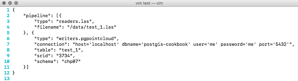
Now, we can download our data. It is recommended to either download it from http://gis5.oit.ohio.gov/geodatadownload/ or to download the sample dataset we have for your use, available at http://www.packtpub.com/support.
First, we need to convert our LAS file to a format that can be used by PDAL. We created a Python script, which reads from a directory of LAS files and generates its corresponding JSON. With this script, we can automate the generation if we have a large directory of files. Also, we chose Python for its simplicity and because you can execute the script regardless of the operating system you are using. To execute the script, run the following in the console (for Windows users, make sure you have the Python interpreter included in the PATH variable):
$ python insert_files.py -f <lasfiles_path>
This script will read each LAS file, and will store within a folder called pipelines all the metadata related to the LAS file that will be inserted into the database.
Now, using PDAL, we execute a for loop to insert LAS files into Postgres:
$ for file in `ls pipelines/*.json`;
do
pdal pipeline $file;
done
This point cloud data is split into three different tables. If we want to merge them, we need to execute the following SQL command:
DROP TABLE IF EXISTS chp07.lidar;
CREATE TABLE chp07.lidar AS WITH patches AS
(
SELECT
pa
FROM "chp07"."N2210595"
UNION ALL
SELECT
pa
FROM "chp07"."N2215595"
UNION ALL
SELECT
pa
FROM "chp07"."N2220595"
)
SELECT
2 AS id,
PC_Union(pa) AS pa
FROM patches;
The postgres-pointcloud extension uses two main point cloud objects as variables: the PcPoint object, which is a point that can have many dimensions, but a minimum of X and Y values that are placed in a space; and the PcPatch object,which is a collection of multiple PcPoints that are close together. According to the documentation of the plugin, it becomes inefficient to store large amounts of points as individual records in a table.
Now that we have all of our data into our database within a single table, if we want to visualize our point cloud data, we need to create a spatial table to be understood by our layer viewer; for instance, QGIS. The point cloud plugin for Postgres has PostGIS integration, so we can transform our PcPatch and PcPoint objects into geometries and use PostGIS functions for analyzing the data:
CREATE TABLE chp07.lidar_patches AS WITH pts AS
(
SELECT
PC_Explode(pa) AS pt
FROM chp07.lidar
)
SELECT
pt::geometry AS the_geom
FROM pts;
ALTER TABLE chp07.lidar_patches ADD COLUMN gid serial;
ALTER TABLE chp07.lidar_patches ADD PRIMARY KEY (gid);
This SQL script performs an inner query, which initially returns a set of PcPoints from the PcPatch using the PC_Explode function. Then, for each point returned, we cast from PcPoint object to a PostGIS geometry object. Finally, we create the gid column and add it to the table as a primary key.
Now, we can view our data using our favorite desktop GIS, as shown in the following image:
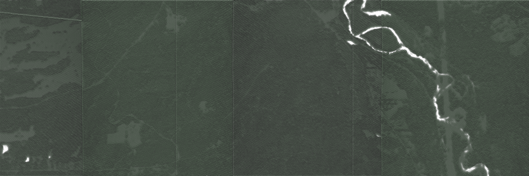
In the previous recipe, Importing LiDAR data, we brought a LiDAR 3D point cloud into PostGIS, creating an explicit 3D dataset from the input. With the data in 3D form, we have the ability to perform spatial queries against it. In this recipe, we will leverage 3D indexes so that our nearest-neighbor search works in all the dimensions our data are in.
We will use the LiDAR data imported in the previous recipe as our dataset of choice. We named that table chp07.lidar. To perform a nearest-neighbor search, we will require an index created on the dataset. Spatial indexes, much like ordinary database table indexes, are similar to book indexes insofar as they help us find what we are looking for faster. Ordinarily, such an index-creation step would look like the following (which we won't run this time):
CREATE INDEX chp07_lidar_the_geom_idx ON chp07.lidar USING gist(the_geom);
A 3D index does not perform as quickly as a 2D index for 2D queries, so a CREATE INDEX query defaults to creating a 2D index. In our case, we want to force the gist to apply to all three dimensions, so we will explicitly tell PostgreSQL to use the n-dimensional version of the index:
CREATE INDEX chp07_lidar_the_geom_3dx ON chp07.lidar USING gist(the_geom gist_geometry_ops_nd);
Note that the approach depicted in the previous code would also work if we had a time dimension or a 3D plus time. Let's load a second 3D dataset and the stream centerlines that we will use in our query:
$ shp2pgsql -s 3734 -d -i -I -W LATIN1 -t 3DZ -g the_geom hydro_line chp07.hydro | PGPASSWORD=me psql -U me -d "postgis-cookbook" -h localhost
This data, as shown in the following image, overlays nicely with our LiDAR point cloud:
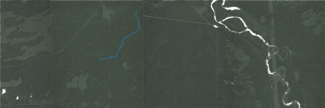
Now, we can build a simple query to retrieve all the LiDAR points within one foot of our stream centerline:
DROP TABLE IF EXISTS chp07.lidar_patches_within; CREATE TABLE chp07.lidar_patches_within AS SELECT chp07.lidar_patches.gid, chp07.lidar_patches.the_geom FROM chp07.lidar_patches, chp07.hydro WHERE ST_3DDWithin(chp07.hydro.the_geom, chp07.lidar_patches.the_geom, 5);
But, this is a little bit of a sloppy approach; we could end up with duplicate LiDAR points, so we will refine our query with LEFT JOIN and SELECT DISTINCT instead, but continue using ST_DWithin as our limiting condition:
DROP TABLE IF EXISTS chp07.lidar_patches_within_distinct; CREATE TABLE chp07.lidar_patches_within_distinct AS SELECT DISTINCT (chp07.lidar_patches.the_geom), chp07.lidar_patches.gid FROM chp07.lidar_patches, chp07.hydro WHERE ST_3DDWithin(chp07.hydro.the_geom, chp07.lidar_patches.the_geom, 5);
Now we can visualize our returned points, as shown in the following image:
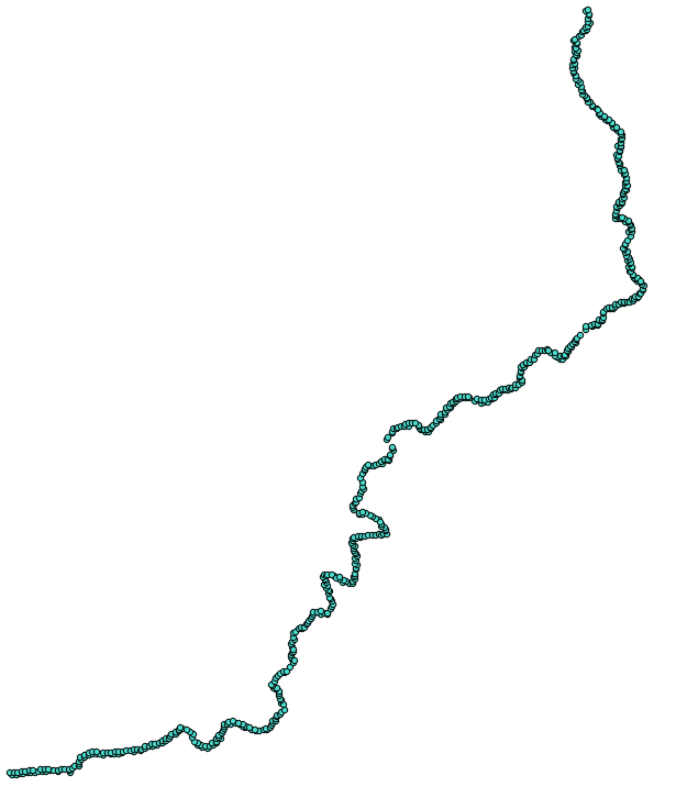
Try this query using ST_DWithin instead of ST_3DDWithin. You'll find an interesting difference in the number of points returned, since ST_DWithin will collect LiDAR points that may be close to our streamline in the XY plane, but not as close when looking at a 3D distance.
You can imagine ST_3DWithin querying within a tunnel around our line. ST_DWithin, by contrast, is going to query a vertical wall of LiDAR points, as it is only searching for adjacent points based on XY distance, ignoring height altogether, and thus gathering up all the points within a narrow wall above and below our points.
In the Detailed building footprints from LiDAR recipe in Chapter 4, Working with Vector Data - Advanced Recipes, we explored the automatic generation of building footprints using LiDAR data. What we were attempting to do was create 2D data from 3D data. In this recipe, we attempt the opposite, in a sense. We start with 2D polygons of building footprints and feed them into a function that extrudes them as 3D polygons.
For this recipe, we will extrude a building footprint of our own making. Let us quickly create a table with a single building footprint, for testing purposes, as follows:
DROP TABLE IF EXISTS chp07.simple_building;
CREATE TABLE chp07.simple_building AS
SELECT 1 AS gid, ST_MakePolygon(
ST_GeomFromText(
'LINESTRING(0 0,2 0, 2 1, 1 1, 1 2, 0 2, 0 0)'
)
) AS the_geom;
It would be beneficial to keep the creation of 3D buildings encapsulated as simply as possible in a function:
CREATE OR REPLACE FUNCTION chp07.threedbuilding(footprint geometry, height numeric) RETURNS geometry AS $BODY$
Our function takes two inputs: the building footprint and a height to extrude to. We can also imagine a function that takes in a third parameter: the height of the base of the building.
To construct the building walls, we will need to first convert our polygons into linestrings and then further separate the linestrings into their individual, two-point segments:
WITH simple_lines AS
(
SELECT
1 AS gid,
ST_MakeLine(ST_PointN(the_geom,pointn),
ST_PointN(the_geom,pointn+1)) AS the_geom
FROM (
SELECT 1 AS gid,
polygon_to_line($1) AS the_geom
) AS a
LEFT JOIN(
SELECT
1 AS gid,
generate_series(1,
ST_NumPoints(polygon_to_line($1))-1
) AS pointn
) AS b
ON a.gid = b.gid
),
The preceding code returns each of the two-point segments of our original shape. For example, for simple_building, the output is as follows:
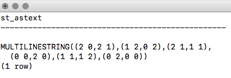
Now that we have a series of individual lines, we can use those to construct the walls of the building. First, we need to recast our 2D lines as 3D using ST_Force3DZ:
threeDlines AS
( SELECT ST_Force3DZ(the_geom) AS the_geom FROM simple_lines ),
The output is as follows:
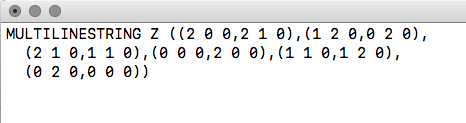
The next step is to break each of those lines from MULTILINESTRING into many LINESTRINGS:
explodedLine AS ( SELECT (ST_Dump(the_geom)).geom AS the_geom FROM threeDLines ),
The output for this is as follows:
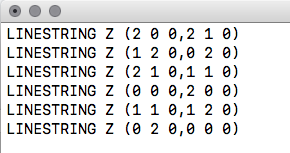
The next step is to construct a line representing the boundary of the extruded wall:
threeDline AS
(
SELECT ST_MakeLine(
ARRAY[
ST_StartPoint(the_geom),
ST_EndPoint(the_geom),
ST_Translate(ST_EndPoint(the_geom), 0, 0, $2),
ST_Translate(ST_StartPoint(the_geom), 0, 0, $2),
ST_StartPoint(the_geom)
]
)
AS the_geom FROM explodedLine
),
Now, we need to convert each linestring to polygon.threeDwall:
threeDwall AS ( SELECT ST_MakePolygon(the_geom) as the_geom FROM threeDline ),
Finally, put in the roof and floor on our building, using the original geometry for the floor (forced to 3D) and a copy of the original geometry translated to our input height:
buildingTop AS ( SELECT ST_Translate(ST_Force3DZ($1), 0, 0, $2) AS the_geom ), -- and a floor buildingBottom AS ( SELECT ST_Translate(ST_Force3DZ($1), 0, 0, 0) AS the_geom ),
We put the walls, roof, and floor together and, during the process, convert this to a 3D MULTIPOLYGON:
wholeBuilding AS
(
SELECT the_geom FROM buildingBottom
UNION ALL
SELECT the_geom FROM threeDwall
UNION ALL
SELECT the_geom FROM buildingTop
),
-- then convert this collecion to a multipolygon
multiBuilding AS
(
SELECT ST_Multi(ST_Collect(the_geom)) AS the_geom FROM
wholeBuilding
),
While we could leave our geometry as a MULTIPOLYGON, we'll do things properly and munge an informal cast to POLYHEDRALSURFACE. In our case, we are already effectively formatted as a POLYHEDRALSURFACE, so we'll just convert our geometry to text with ST_AsText, replace the word with POLYHEDRALSURFACE, and then convert our text back to geometry with ST_GeomFromText:
textBuilding AS ( SELECT ST_AsText(the_geom) textbuilding FROM multiBuilding ), textBuildSurface AS ( SELECT ST_GeomFromText(replace(textbuilding, 'MULTIPOLYGON',
'POLYHEDRALSURFACE')) AS the_geom FROM textBuilding ) SELECT the_geom FROM textBuildSurface
Finally, the entire function is:
CREATE OR REPLACE FUNCTION chp07.threedbuilding(footprint geometry,
height numeric)
RETURNS geometry AS
$BODY$
-- make our polygons into lines, and then chop up into individual line segments
WITH simple_lines AS
(
SELECT 1 AS gid, ST_MakeLine(ST_PointN(the_geom,pointn),
ST_PointN(the_geom,pointn+1)) AS the_geom
FROM (SELECT 1 AS gid, polygon_to_line($1) AS the_geom ) AS a
LEFT JOIN
(SELECT 1 AS gid, generate_series(1,
ST_NumPoints(polygon_to_line($1))-1) AS pointn
) AS b
ON a.gid = b.gid
),
-- convert our lines into 3D lines, which will set our third coordinate to 0 by default
threeDlines AS
(
SELECT ST_Force3DZ(the_geom) AS the_geom FROM simple_lines
),
-- now we need our lines as individual records, so we dump them out using ST_Dump, and then just grab the geometry portion of the dump
explodedLine AS
(
SELECT (ST_Dump(the_geom)).geom AS the_geom FROM threeDLines
),
-- Next step is to construct a line representing the boundary of the extruded "wall"
threeDline AS
(
SELECT ST_MakeLine(
ARRAY[
ST_StartPoint(the_geom),
ST_EndPoint(the_geom),
ST_Translate(ST_EndPoint(the_geom), 0, 0, $2),
ST_Translate(ST_StartPoint(the_geom), 0, 0, $2),
ST_StartPoint(the_geom)
]
)
AS the_geom FROM explodedLine
),
-- we convert this line into a polygon
threeDwall AS
(
SELECT ST_MakePolygon(the_geom) as the_geom FROM threeDline
),
-- add a top to the building
buildingTop AS
(
SELECT ST_Translate(ST_Force3DZ($1), 0, 0, $2) AS the_geom
),
-- and a floor
buildingBottom AS
(
SELECT ST_Translate(ST_Force3DZ($1), 0, 0, 0) AS the_geom
),
-- now we put the walls, roof, and floor together
wholeBuilding AS
(
SELECT the_geom FROM buildingBottom
UNION ALL
SELECT the_geom FROM threeDwall
UNION ALL
SELECT the_geom FROM buildingTop
),
-- then convert this collecion to a multipolygon
multiBuilding AS
(
SELECT ST_Multi(ST_Collect(the_geom)) AS the_geom FROM wholeBuilding
),
-- While we could leave this as a multipolygon, we'll do things properly and munge an informal cast
-- to polyhedralsurfacem which is more widely recognized as the appropriate format for a geometry like
-- this. In our case, we are already formatted as a polyhedralsurface, minus the official designation,
-- so we'll just convert to text, replace the word MULTIPOLYGON with POLYHEDRALSURFACE and then convert
-- back to geometry with ST_GeomFromText
textBuilding AS
(
SELECT ST_AsText(the_geom) textbuilding FROM multiBuilding
),
textBuildSurface AS
(
SELECT ST_GeomFromText(replace(textbuilding, 'MULTIPOLYGON',
'POLYHEDRALSURFACE')) AS the_geom FROM textBuilding
)
SELECT the_geom FROM textBuildSurface
;
$BODY$
LANGUAGE sql VOLATILE
COST 100;
ALTER FUNCTION chp07.threedbuilding(geometry, numeric)
OWNER TO me;
Now that we have a 3D-building extrusion function, we can easily extrude our building footprint with our nicely encapsulated function:
DROP TABLE IF EXISTS chp07.threed_building; CREATE TABLE chp07.threed_building AS SELECT chp07.threeDbuilding(the_geom, 10) AS the_geom FROM chp07.simple_building;
We can apply this function to a real building footprint dataset (available in our data directory), in which case, if we have a height field, we can extrude according to it:
shp2pgsql -s 3734 -d -i -I -W LATIN1 -g the_geom building_footprints\chp07.building_footprints | psql -U me -d postgis-cookbook \
-h <HOST> -p <PORT>
DROP TABLE IF EXISTS chp07.build_footprints_threed; CREATE TABLE chp07.build_footprints_threed AS SELECT gid, height, chp07.threeDbuilding(the_geom, height) AS the_geom FROM chp07.building_footprints;
The resulting output gives us a nice, extruded set of building footprints, as shown in the following image:
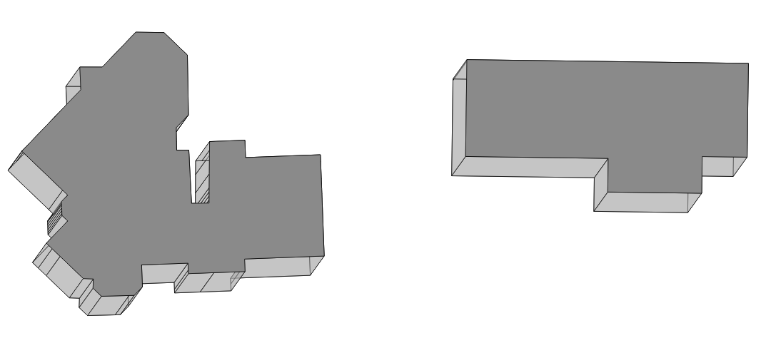
The Detailed building footprints from LiDAR recipe in Chapter 4, Working with Vector Data - Advanced Recipes, explores the extraction of building footprints from LiDAR. A complete workflow could be envisioned, which extracts building footprints from LiDAR and then reconstructs polygon geometries using the current recipe, thus converting point clouds to surfaces, combining the current recipe with the one referenced previously.
PostGIS 2.1 brought a lot of really cool additional functionality to PostGIS. Operations on PostGIS raster types are among the more important improvements that come with PostGIS 2.1. A quieter and equally potent game changer was the addition of the SFCGAL library as an optional extension to PostGIS. According to the website http://sfcgal.org/, SFCGAL is a C++ wrapper library around CGAL with the aim of supporting ISO 19107:2013 and OGC Simple Features Access 1.2 for 3D operations.
From a practical standpoint, what does this mean? It means that PostGIS is moving toward a fully functional 3D environment, from representation of the geometries themselves and the operations on those 3D geometries. More information is available at http://postgis.net/docs/reference.html#reference_sfcgal.
This and several other recipes will assume that you have a version of PostGIS installed with SFCGAL compiled and enabled. Doing so enables the following functions:
For this recipe, we'll use ST_Extrude in much the same way we used our own custom-built function in the previous recipe, Constructing and serving buildings 2.5D. The advantage over the previous recipe is that we are not required to have the SFCGAL library compiled in PostGIS. The advantage to this recipe is that we have more control over the extrusion process; that is, we can extrude in all three dimensions.
ST_Extrude returns a geometry, specifically a polyhedral surface. It requires four parameters: an input geometry and the extrusion amount along the X, Y, and Z axes:
DROP TABLE IF EXISTS chp07.buildings_extruded; CREATE TABLE chp07.buildings_extruded AS SELECT gid, ST_CollectionExtract(ST_Extrude(the_geom, 20, 20, 40), 3) as the_geom FROM chp07.building_footprints
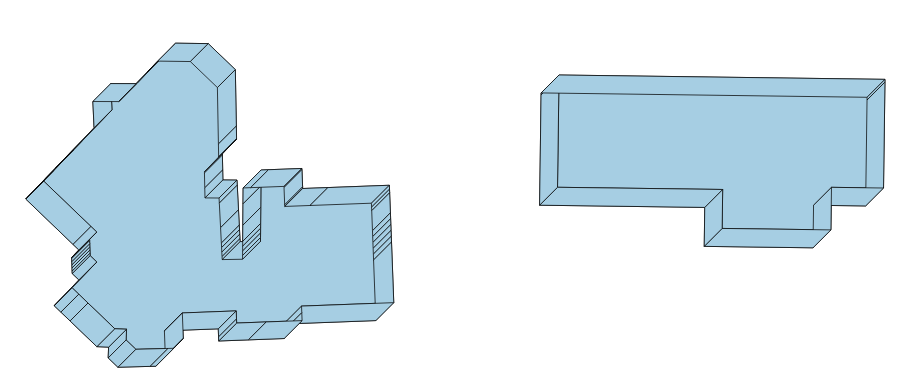
And so, with the help of the Constructing and serving buildings 2.5D recipe, we get our extruded buildings, but with some additional flexibility.
Sources of 3D information are not only generated from LiDAR, nor are they purely synthesized from 2D geometries and associated attributes as in the Constructing and serving buildings 2.5D and Using ST_Extrude to extrude building footprints recipes, but they can also be created from the principles of computer vision as well. The process of calculating 3D information from the association of related keypoints between images is known as SfM.
As a computer vision concept, we can leverage SfM to generate 3D information in ways similar to how the human mind perceives the world in 3D, and further store and process that information in a PostGIS database.
A number of open source projects have matured to deal with solving SfM problems. Popular among these are Bundler, which can be found at http://phototour.cs.washington.edu/bundler/, and VisualSFM at http://ccwu.me/vsfm/. Binaries exist for multiple platforms for these tools, including versions. The nice thing about such projects is that a simple set of photos can be used to reconstruct 3D scenes.
For our purposes, we will use VisualSFM and skip the installation and configuration of this software. The reason for this is that SfM is beyond the scope of a PostGIS book to cover in detail, and we will focus on how we can use the data in PostGIS.
It is important to understand that SfM techniques, while highly effective, have certain limitations in the kinds of imagery that can be effectively processed into point clouds. The techniques are dependent upon finding matches between subsequent images and thus can have trouble processing images that are smooth, are missing the camera's embedded Exchangeable Image File Format (EXIF) information, or are from cell phone cameras.
We will start processing an image series into a point cloud with a photo series that we know largely works, but as you experiment with SfM, you can feed in your own photo series. Good tips on how to create a photo series that will result in a 3D model can be found at https://www.youtube.com/watch?v=IStU-WP2XKs&t=348s and http://www.cubify.com/products/capture/photography_tips.aspx.
Download VisualSFM from http://ccwu.me/vsfm/. In a console terminal, execute the following:
Visualsfm <IMAGES_FOLDER>
VisualSFM will start rendering the 3D, model using as input a folder with images. It will take a couple of hours to process. Then, when it finishes, it will return a point cloud file.
We can view this data in a program such as MeshLab at http://meshlab.sourceforge.net/. A good tutorial on using MeshLab to view point clouds can be found at http://www.cse.iitd.ac.in/~mcs112609/Meshlab%20Tutorial.pdf.
The following image shows what our point cloud looks like when viewed in MeshLab:
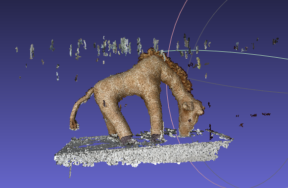
In the VisualSFM output, there is a file with the extension .ply, for example, giraffe.ply (included in the source code for this chapter). If you open this file in a text editor, it will look something like the following:
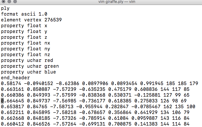
This is the header portion of our file. It specifies the .ply format, the encoding format ascii 1.0, the number of vertices, and then the column names for all the data returned: x, y, z, nx, ny, nz, red, green, and blue.
For importing into PostGIS, we will import all the fields, but will focus on x, y, and z for our point cloud, as well as look at color. For our purposes, this file specifies relative x, y, and z coordinates, and the color of each of those points in channels red, green, and blue. These colors are 24-bit colors—and thus they can have integer values between 0 and 255.
For the remainder of the recipe, we will create a PDAL pipeline, modifying the JSON structure reader to be a .ply file. Check the recipe for Importing LiDAR data in this chapter to see how to create a PDAL pipeline:
{ "pipeline": [{ "type": "readers.ply", "filename": "/data/giraffe/giraffe.ply" }, { "type": "writers.pgpointcloud", "connection": "host='localhost' dbname='postgis-cookbook' user='me'
password='me' port='5432'", "table": "giraffe", "srid": "3734", "schema": "chp07" }] }
Then we execute in the Terminal:
$ pdal pipeline giraffe.json"
This output will serve us for input in the next recipe.
Entering 3D data in a PostGIS database is not nearly as interesting if we have no capacity for extracting the data back out in some useable form. One way to approach this problem is to leverage the PostGIS ability to write 3D tables to the X3D format.
X3D is an XML standard for displaying 3D data and works well via the web. For those familiar with Virtual Reality Modeling Language (VRML), X3D is the next generation of that.
To view X3D in the browser, a user has the choice of a variety of plugins, or they can leverage JavaScript APIs to enable viewing. We will perform the latter, as it requires no user configuration to work. We will use X3DOM's JavaScript framework to accomplish this. X3DOM is a demonstration of the integration of HTML5 and 3D and uses Web Graphics Library (WebGL); (https://en.wikipedia.org/wiki/WebGL) to allow rendering and interaction with 3D content in the browser. This means that our data will not get displayed in browsers that are not WebGL compatible.
We will be using the point cloud from the previous example to serve in X3D format. PostGIS documentation on X3D includes an example of using the ST_AsX3D function to output the formatted X3D code:
COPY(WITH pts AS (SELECT PC_Explode(pa) AS pt FROM chp07.giraffe) SELECT ' <X3D xmlns="http://www.web3d.org/specifications/x3d-namespace" showStat="false" showLog="false" x="0px" y="0px" width="800px" height="600px"> <Scene> <Transform> <Shape>' || ST_AsX3D(ST_Union(pt::geometry)) ||'</Shape> </Transform> </Scene> </X3D>' FROM pts) TO STDOUT WITH CSV;
We included the copy to STDOUT WITH CSV to make a dump in raw code. The user is able to save this query as an SQL script file and execute it from the console in order to dump the result into a file. For instance:
$ psql -U me -d postgis-cookbook -h localhost -f "x3d_query.sql" > result.html
This example, while complete in serving the pure X3D, needs additional code to allow in-browser viewing. We do so by including style sheets, and the appropriate X3DOM includes the headers of an XHTML document:
<link rel="stylesheet" type="text/css" href="http://x3dom.org/x3dom/example/x3dom.css" />
<script type="text/javascript" src="http://x3dom.org/x3dom/example/x3dom.js"></script>
The full query to generate the XHTML of X3D data is as follows:
COPY(WITH pts AS (
SELECT PC_Explode(pa) AS pt FROM chp07.giraffe
)
SELECT regexp_replace('
<!DOCTYPE html PUBLIC "-//W3C//DTD XHTML 1.0 Strict//EN" "http://www.w3.org/TR/xhtml1/DTD/xhtml1-strict.dtd">
<html xmlns="http://www.w3.org/1999/xhtml">
<head>
<meta http-equiv="X-UA-Compatible" content="chrome=1" />
<meta http-equiv="Content-Type" content="text/html;charset=utf-8"/>
<title>Point Cloud in a Browser</title>
<link rel="stylesheet" type="text/css"
href="http://x3dom.org/x3dom/example/x3dom.css" />
<script type="text/javascript"
src="http://x3dom.org/x3dom/example/x3dom.js">
</script>
</head>
<body>
<h1>Point Cloud in the Browser</h1>
<p>
Use mouse to rotate, scroll wheel to zoom, and control
(or command) click to pan.
</p>
<X3D xmlns="http://www.web3d.org/specifications/x3d-namespace
showStat="false" showLog="false" x="0px" y="0px" width="800px"
height="600px">
<Scene>
<Transform>
<Shape>' || ST_AsX3D(ST_Union(pt::geometry)) || '</Shape>
</Transform>
</Scene>
</X3D>
</body>
</html>', E'[\\n\\r]+','', 'g')
FROM pts)TO STDOUT;
If we open the .html file in our favorite browser, we will get the following:
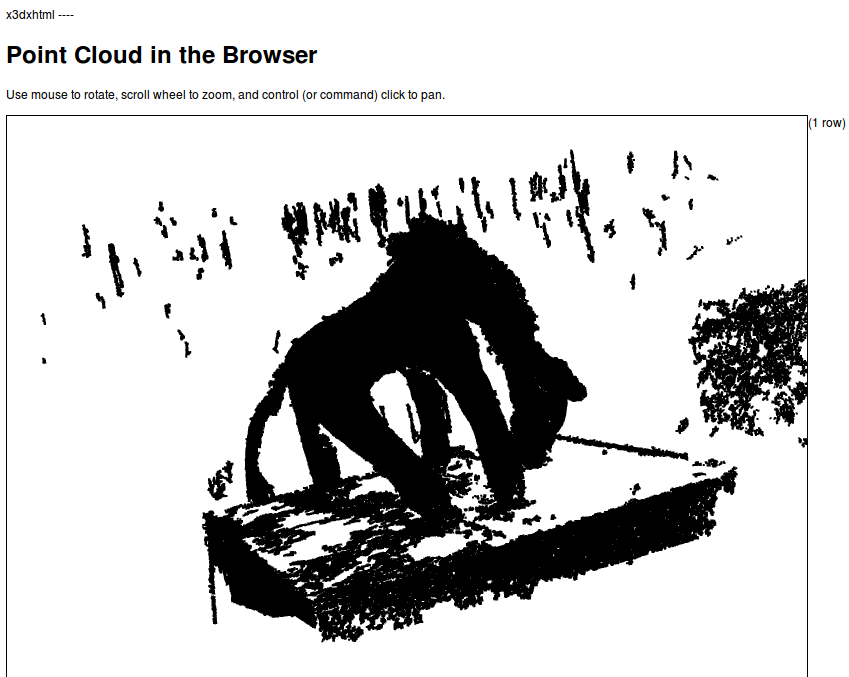
One might want to use this X3D conversion as a function, feeding geometry into a function and getting a page in return. In this way, we can reuse the code easily for other tables. Embodied in a function, X3D conversion is as follows:
CREATE OR REPLACE FUNCTION AsX3D_XHTML(geometry) RETURNS character varying AS $BODY$ SELECT regexp_replace( ' <!DOCTYPE html PUBLIC "-//W3C//DTD XHTML 1.0 Strict//EN"
"http://www.w3.org/TR/xhtml1/DTD/xhtml1-strict.dtd"> <html xmlns= "http://www.w3.org/1999/xhtml"> <head> <meta http-equiv="X-UA-Compatible" content="chrome=1"/> <meta http-equiv="Content-Type" content="text/html;charset=utf-8"/> <title>Point Cloud in a Browser</title> <link rel="stylesheet" type="text/css"
href="http://x3dom.org/x3dom/example/x3dom.css"/> <script type="text/javascript"
src="http://x3dom.org/x3dom/example/x3dom.js">
</script> </head> <body> <h1>Point Cloud in the Browser</h1> <p> Use mouse to rotate, scroll wheel to zoom, and control
(or command) click to pan. </p> <X3D xmlns="http://www.web3d.org/specifications/x3d-namespace"
showStat="false" showLog="false" x="0px" y="0px" width="800px"
height="600px"> <Scene> <Transform> <Shape>'|| ST_AsX3D($1) || '</Shape> </Transform> </Scene> </X3D> </body> </html> ', E'[\\n\\r]+' , '' , 'g' ) As x3dXHTML; $BODY$ LANGUAGE sql VOLATILE COST 100;
In order for the function to work, we need to first use ST_UNION on the geometry parameter to pass to the AsX3D_XHTML function:
copy(
WITH pts AS (
SELECT
PC_Explode(pa) AS pt
FROM giraffe
)
SELECT AsX3D_XHTML(ST_UNION(pt::geometry)) FROM pts) to stdout;
We can now very simply generate the appropriate XHTML directly from the command line or a web framework.
The rapid development of Unmanned Aerial Systems (UAS), also known as Unmanned Aerial Vehicles (UAVs), as data collectors is revolutionizing remote data collection in all sectors. Barriers to wider adoption outside military sectors include regulatory frameworks preventing their flight in some nations, such as, the United States, and the lack of open source implementations of post-processing software. In the next four recipes, we'll attempt preliminary solutions to the latter of these two barriers.
For this recipe, we will be using the metadata from a UAV flight in Seneca County, Ohio, by the Ohio Department of Transportation to map the coverage of the flight. This is included in the code folder for this chapter.
The basic idea for this recipe is to estimate the field of view of the UAV camera, generate a 3D pyramid that represents that field of view, and use the flight ephemeris (bearing, pitch, and roll) to estimate ground coverage.
The metadata or ephemeris we have for the flight includes the bearing, pitch, and roll of the UAS, in addition to its elevation and location:
To translate these ephemeris into PostGIS terms, we'll assume the following:
In order to perform our analysis, we require external functions. These functions can be downloaded from https://github.com/smathermather/postgis-etc/tree/master/3D.
We will use patched versions of ST_RotateX, ST_RotateY (ST_RotateX.sql, and ST_RotateY.sql), which allow us to rotate geometries around an input point, as well as a function for calculating our field of view, pyramidMaker.sql. Future versions of PostGIS will include these versions of ST_RotateX and ST_RotateY built in. We have another function, ST_RotateXYZ, which is built upon these and will also simplify our code by allowing us to specify three axes at the same time for rotation.
For the final step, we'll need the capacity to perform volumetric intersection (the 3D equivalent of intersection). For this, we'll use volumetricIntersection.sql, which allows us to just return the volumetric portion of the intersection as a triangular irregular network (TIN).
We will install the functions as follows:
psql -U me -d postgis_cookbook -f ST_RotateX.sql psql -U me -d postgis_cookbook -f ST_RotateY.sql psql -U me -d postgis_cookbook -f ST_RotateXYZ.sql psql -U me -d postgis_cookbook -f pyramidMaker.sql psql -U me -d postgis_cookbook -f volumetricIntersection.sql
In order to calculate the viewing footprint, we will calculate a rectangular pyramid descending from the viewpoint to the ground. This pyramid will need to point to the left and right of the nadir according to the UAS's roll, forward or backward from the craft according to its pitch, and be oriented relative to the direction of movement of the craft according to its bearing.
The pyramidMaker function will construct our pyramid for us and ST_RotateXYZ will rotate the pyramid in the direction we need to compensate for roll, pitch, and bearing.
The following image is an example map of such a calculated footprint for a single image. Note the slight roll to the left for this example, resulting in an asymmetric-looking pyramid when viewed from above:
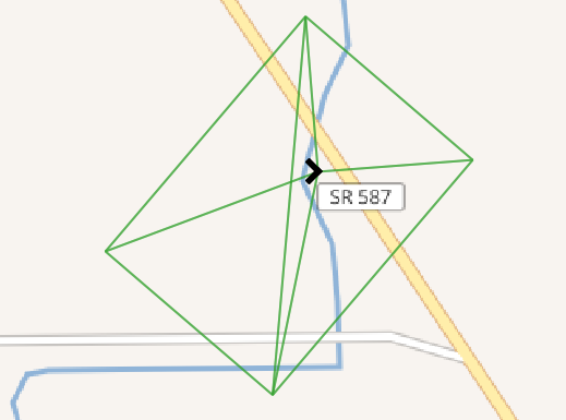
The total track for the UAS flight overlayed on a contour map is shown in the following image:
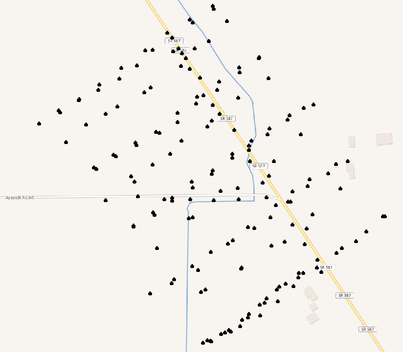
We will write a function to calculate our footprint pyramid. To input to the function, we'll need the position of the UAS as geometry (origin), the pitch, bearing, and roll, as well as the field of view angle in x and y for the camera. Finally, we'll need the relative height of the craft above ground:
CREATE OR REPLACE FUNCTION chp07.pbr(origin geometry, pitch numeric, bearing numeric, roll numeric, anglex numeric, angley numeric, height numeric) RETURNS geometry AS $BODY$
Our pyramid function assumes that we know what the base size of our pyramid is. We don't know this initially, so we'll calculate its size based on the field of view angle of the camera and the height of the craft:
WITH widthx AS ( SELECT height / tan(anglex) AS basex ), widthy AS ( SELECT height / tan(angley) AS basey ),
Now, we have enough information to construct our pyramid:
iViewCone AS (
SELECT pyramidMaker(origin, basex::numeric, basey::numeric, height)
AS the_geom
FROM widthx, widthy
),
We will require the following code to rotate our view relative to pitch, roll, and bearing:
iViewRotated AS (
SELECT ST_RotateXYZ(the_geom, pi() - pitch, 0 - roll, pi() -
bearing, origin) AS the_geom FROM iViewCone
)
SELECT the_geom FROM iViewRotated
The whole function is as follows:
CREATE OR REPLACE FUNCTION chp07.pbr(origin geometry, pitch numeric,
bearing numeric, roll numeric, anglex numeric, angley numeric,
height numeric)
RETURNS geometry AS
$BODY$
WITH widthx AS
(
SELECT height / tan(anglex) AS basex
),
widthy AS
(
SELECT height / tan(angley) AS basey
),
iViewCone AS (
SELECT pyramidMaker(origin, basex::numeric, basey::numeric, height)
AS the_geom
FROM widthx, widthy
),
iViewRotated AS (
SELECT ST_RotateXYZ(the_geom, pi() - pitch, 0 - roll, pi() -
bearing, origin) AS the_geom FROM iViewCone
)
SELECT the_geom FROM iViewRotated
;
$BODY$
LANGUAGE sql VOLATILE
COST 100;
Now, to use our function, let us import the UAS positions from the uas_locations shapefile included in the source for this chapter:
shp2pgsql -s 3734 -W LATIN1 uas_locations_altitude_hpr_3734 uas_locations | \PGPASSWORD=me psql -U me -d postgis-cookbook -h localhost
Now, it is possible to calculate an estimated footprint for each UAS position:
DROP TABLE IF EXISTS chp07.viewshed; CREATE TABLE chp07.viewshed AS SELECT 1 AS gid, roll, pitch, heading, fileName, chp07.pbr(ST_Force3D(geom), radians(0)::numeric, radians(heading)::numeric, radians(roll)::numeric, radians(40)::numeric, radians(50)::numeric,
( (3.2808399 * altitude_a) - 838)::numeric) AS the_geom FROM uas_locations;
If you import this with your favorite desktop GIS, such as QGIS, you will be able to see the following:
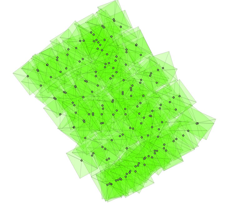
With a terrain model, we can go a step deeper in this analysis. Since our UAS footprints are volumetric, we will first load the terrain model. We will load this from a .backup file included in the source code for this chapter:
pg_restore -h localhost -p 8000 -U me -d "postgis-cookbook" \ --schema chp07 --verbose "lidar_tin.backup"
Next, we will create a smaller version of our viewshed table:
DROP TABLE IF EXISTS chp07.viewshed; CREATE TABLE chp07.viewshed AS SELECT 1 AS gid, roll, pitch, heading, fileName, chp07.pbr(ST_Force3D(geom), radians(0)::numeric, radians(heading)::numeric, radians(roll) ::numeric, radians(40)::numeric, radians(50)::numeric, 1000::numeric) AS the_geom FROM uas_locations WHERE fileName = 'IMG_0512.JPG';
If you import this with your favorite desktop GIS, such as QGIS, you will be able to see the following:
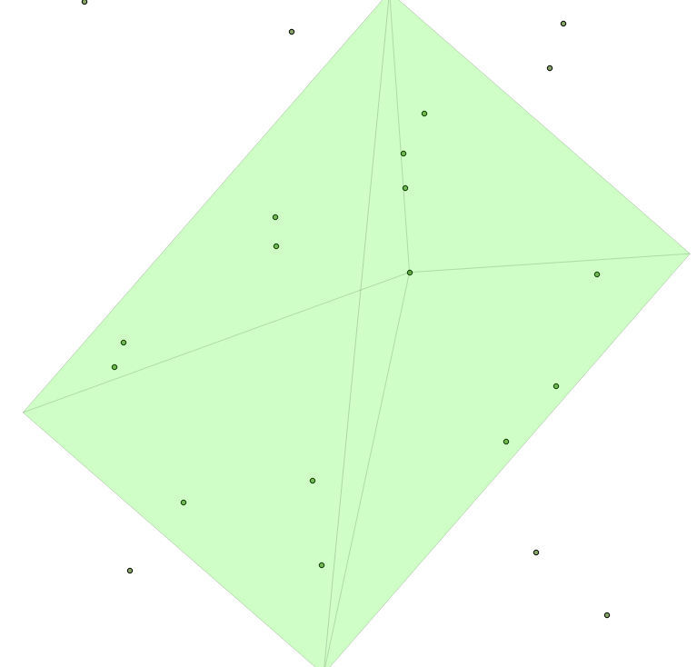
We will use the techniques we've used in the previous recipe named Creating arbitrary 3D objects for PostGIS learn how to create and import a UAV-derived point cloud in PostGIS.
One caveat before we begin is that while we will be working with geospatial data, we will be doing so in relative space, rather than a known coordinate system. In other words, this approach will calculate our dataset in an arbitrary coordinate system. ST_Affine could be used in combination with the field measurements of locations to transform our data into a known coordinate system, but this is beyond the scope of this book.
Much like with the Creating arbitrary 3D objects for PostGIS recipe, we will be taking an image series and converting it into a point cloud. In this case, however, our image series will be from UAV imagery. Download the image series included in the code folder for this chapter, uas_flight, and feed it into VisualSFM (check http://ccwu.me/vsfm/for more information on how to use this tool); in order to retrieve a point cloud, name it uas_points.ply (this file is also included in this folder in case you would rather use it).
The input for PostGIS is the same as before. Create a JSON file and use PDAL store it into the database:
{
"pipeline": [{
"type": "readers.ply",
"filename": "/data/uas_flight/uas_points.ply"
}, {
"type": "writers.pgpointcloud",
"connection": "host='localhost' dbname='postgis-cookbook' user='me'
password='me' port='5432'",
"table": "uas",
"schema": "chp07"
}]
}
Now, we copy data from the point cloud into our table. Refer to the Importing LiDAR data recipe in this chapter to verify the pointcloud extension object representation:
$ pdal pipeline uas_points.json
This data, as viewed in MeshLab (http://www.meshlab.net/) from the .ply file, is pretty interesting:
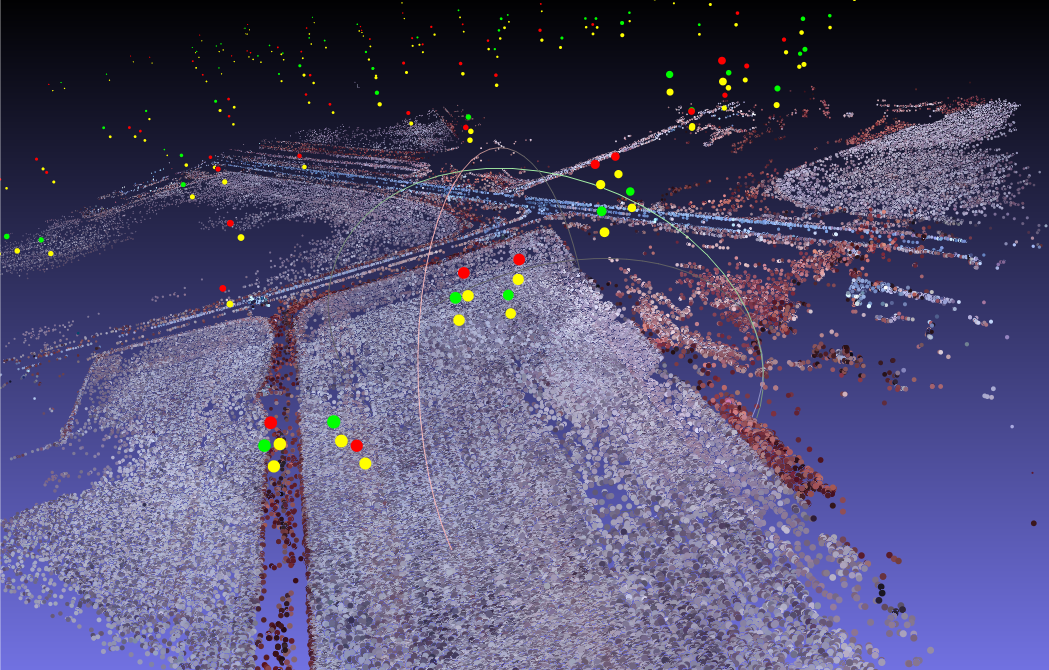
The original data is color infrared imagery, so vegetation shows up red, and farm fields and roads as gray. Note the bright colors in the sky; those are camera position points that we'll need to filter out.
The next step is to generate orthographic imagery from this data.
The photogrammetry example would be incomplete if we did not produce a digital terrain model from our inputs. A fully rigorous solution where the input point cloud would be classified into ground points, building points, and vegetation points is not feasible here, but this recipe will provide the basic framework for accomplishing such a solution.
In this recipe, we will create a 3D TIN, which will represent the surface of the point cloud.
Before we start, ST_DelaunayTriangles is available only in PostGIS 2.1 using GEOS 3.4. This is one of the few recipes in this book to require such advanced versions of PostGIS and GEOS.
ST_DelaunayTriangles will calculate a 3D TIN with the correct flag: geometry ST_DelaunayTriangles (geometry g1, float tolerance, int4 flags):
DROP TABLE IF EXISTS chp07.uas_tin; CREATE TABLE chp07.uas_tin AS WITH pts AS ( SELECT PC_Explode(pa) AS pt FROM chp07.uas_flights ) SELECT ST_DelaunayTriangles(ST_Union(pt::geometry), 0.0, 2) AS the_geom FROM pts;
Now, we have a full TIN of a digital surface model at our disposal:
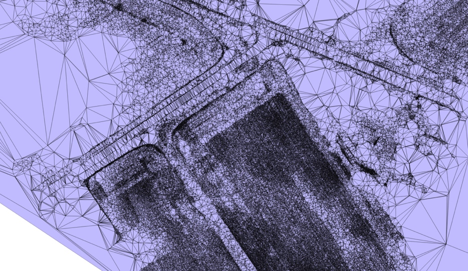
In this chapter, we will cover the following topics:
There are several ways to write PostGIS programs, and in this chapter we will see a few of them. You will mainly use the Python language throughout this chapter. Python is a fantastic language with a plethora of GIS and scientific libraries that can be combined with PostGIS to write awesome geospatial applications.
If you are new to Python, you can quickly get productive with these excellent web resources:
You can combine Python with some excellent and popular libraries, such as:
The recipes in this chapter will cover some other useful geospatial Python libraries that are worthy of being looked at if you are developing a geospatial application. Under these Python libraries, the following libraries are included:
In the first recipe, you will write a program that uses Python and its utilities such as psycopg, requests, and simplejson to fetch weather data from the web and import it in PostGIS.
In the second recipe, we will drive you to use Python and the GDAL OGR Python bindings library to create a script for geocoding a list of place names using one of the GeoNames web services.
You will then write a Python function for PostGIS using the PL/Python language to query the http://openweathermap.org/ web services, already used in the first recipe, to calculate the weather for a PostGIS geometry from within a PostgreSQL function.
In the fourth recipe, you will create two PL/pgSQL PostGIS functions that will let you perform geocoding and reverse geocoding using the GeoNames datasets.
After this, there is a recipe in which you will use the OpenStreetMap street datasets imported in PostGIS to implement a very basic Python class in order to provide a geocode implementation to the class's consumer using PostGIS trigram support.
The sixth recipe will show you how to create a PL/Python function using the geopy library to geocode addresses using a web geocoding API such as Google Maps, Yahoo! Maps, Geocoder, GeoNames, and others.
In the last recipe of this chapter, you will create a Python script to import data from the netCDF format to PostGIS using the GDAL Python bindings.
Let's see some notes before starting with the recipes in this chapter.
If you are using Linux or macOS, follow these steps:
$ cd ~/virtualenvs
$ virtualenv --no-site-packages postgis-cb-env
$ source postgis-cb-env/bin/activate
$ pip install simplejson
$ pip install psycopg2
$ pip install numpy
$ pip install requests
$ pip install gdal
$ pip install geopy
$ ls /home/capooti/virtualenv/postgis-cb-env/lib/
python2.7/site-packages
If you are wondering what is going on with the previous command lines, then virtualenv is a tool that will be used to create isolated Python environments, and you can find more information about this tool at http://www.virtualenv.org, while pip (http://www.pip-installer.org) is a package management system used to install and manage software packages written in Python.
If you are using Windows, follow these steps:
> python ez_setup.py
> python get-pip.py
> pip install requests
> pip install geopy
In this recipe, you will use Python combined with Psycopg, the most popular PostgreSQL database library for Python, in order to write some data to PostGIS using the SQL language.
You will write a procedure to import weather data for the most populated US cities. You will import such weather data from http://www.openweatherdata.org/, which is a web service that provides free weather data and a forecast API. The procedure you are going to write will iterate each major USA city and get the actual temperature for it from the closest weather stations using the http://www.openweatherdata.org/ web service API, getting the output in JSON format. (In case you are new to the JSON format, you can find details about it at http://www.json.org/.)
You will also generate a new PostGIS layer with the 10 closest weather stations to each city.
postgis_cookbook=# CREATE SCHEMA chp08;
$ ogr2ogr -f PostgreSQL -s_srs EPSG:4269 -t_srs EPSG:4326
-lco GEOMETRY_NAME=the_geom -nln chp08.cities
PG:"dbname='postgis_cookbook' user='me'
password='mypassword'" -where "POP_2000 $ 100000" citiesx020.shp
postgis_cookbook=# ALTER TABLE chp08.cities
ADD COLUMN temperature real;
$ source postgis-cb-env/bin/activate
Carry out the following steps:
CREATE TABLE chp08.wstations
(
id bigint NOT NULL,
the_geom geometry(Point,4326),
name character varying(48),
temperature real,
CONSTRAINT wstations_pk PRIMARY KEY (id )
);
{
"message": "accurate",
"cod": "200",
"count": 10,
"list": [
{
"id": 529315,
"name": "Marinki",
"coord": {
"lat": 55.0944,
"lon": 37.03
},
"main": {
"temp": 272.15,
"pressure": 1011,
"humidity": 80,
"temp_min": 272.15,
"temp_max": 272.15
}, "dt": 1515114000,
"wind": {
"speed": 3,
"deg": 140
},
"sys": {
"country": ""
},
"rain": null,
"snow": null,
"clouds": {
"all": 90
},
"weather": [
{
"id": 804,
"main": "Clouds",
"description": "overcast clouds",
"icon": "04n"
}
]
},
import sys
import requests
import simplejson as json
import psycopg2
def GetWeatherData(lon, lat, key):
"""
Get the 10 closest weather stations data for a given point.
"""
# uri to access the JSON openweathermap web service
uri = (
'https://api.openweathermap.org/data/2.5/find?
lat=%s&lon=%s&cnt=10&appid=%s'
% (lat, lon, key))
print 'Fetching weather data: %s' % uri
try:
data = requests.get(uri)
print 'request status: %s' % data.status_code
js_data = json.loads(data.text)
return js_data['list']
except:
print 'There was an error getting the weather data.'
print sys.exc_info()[0]
return []
def AddWeatherStation(station_id, lon, lat, name, temperature):
"""
Add a weather station to the database, but only if it does
not already exists.
"""
curws = conn.cursor()
curws.execute('SELECT * FROM chp08.wstations WHERE id=%s',
(station_id,))
count = curws.rowcount
if count==0: # we need to add the weather station
curws.execute(
"""INSERT INTO chp08.wstations (id, the_geom, name,
temperature) VALUES (%s, ST_GeomFromText('POINT(%s %s)',
4326), %s, %s)""",
(station_id, lon, lat, name, temperature)
)
curws.close()
print 'Added the %s weather station to the database.' % name
return True
else: # weather station already in database
print 'The %s weather station is already in the database.' % name
return False
# program starts here
# get a connection to the database
conn = psycopg2.connect('dbname=postgis_cookbook user=me
password=password')
# we do not need transaction here, so set the connection
# to autocommit mode
conn.set_isolation_level(0)
# open a cursor to update the table with weather data
cur = conn.cursor()
# iterate all of the cities in the cities PostGIS layer,
# and for each of them grap the actual temperature from the
# closest weather station, and add the 10
# closest stations to the city to the wstation PostGIS layer
cur.execute("""SELECT ogc_fid, name,
ST_X(the_geom) AS long, ST_Y(the_geom) AS lat
FROM chp08.cities;""")
for record in cur:
ogc_fid = record[0]
city_name = record[1]
lon = record[2]
lat = record[3]
stations = GetWeatherData(lon, lat, 'YOURKEY')
print stations
for station in stations:
print station
station_id = station['id']
name = station['name']
# for weather data we need to access the 'main' section in the
# json 'main': {'pressure': 990, 'temp': 272.15, 'humidity': 54}
if 'main' in station:
if 'temp' in station['main']:
temperature = station['main']['temp']
else:
temperature = -9999
# in some case the temperature is not available
# "coord":{"lat":55.8622,"lon":37.395}
station_lat = station['coord']['lat']
station_lon = station['coord']['lon']
# add the weather station to the database
AddWeatherStation(station_id, station_lon, station_lat,
name, temperature)
# first weather station from the json API response is always
# the closest to the city, so we are grabbing this temperature
# and store in the temperature field in cities PostGIS layer
if station_id == stations[0]['id']:
print 'Setting temperature to %s for city %s'
% (temperature, city_name)
cur2 = conn.cursor()
cur2.execute(
'UPDATE chp08.cities SET temperature=%s WHERE ogc_fid=%s',
(temperature, ogc_fid))
cur2.close()
# close cursor, commit and close connection to database
cur.close()
conn.close()
(postgis-cb-env)$ python get_weather_data.py
Added the PAMR weather station to the database.
Setting temperature to 268.15 for city Anchorage
Added the PAED weather station to the database.
Added the PANC weather station to the database.
...
The KMFE weather station is already in the database.
Added the KOPM weather station to the database.
The KBKS weather station is already in the database.
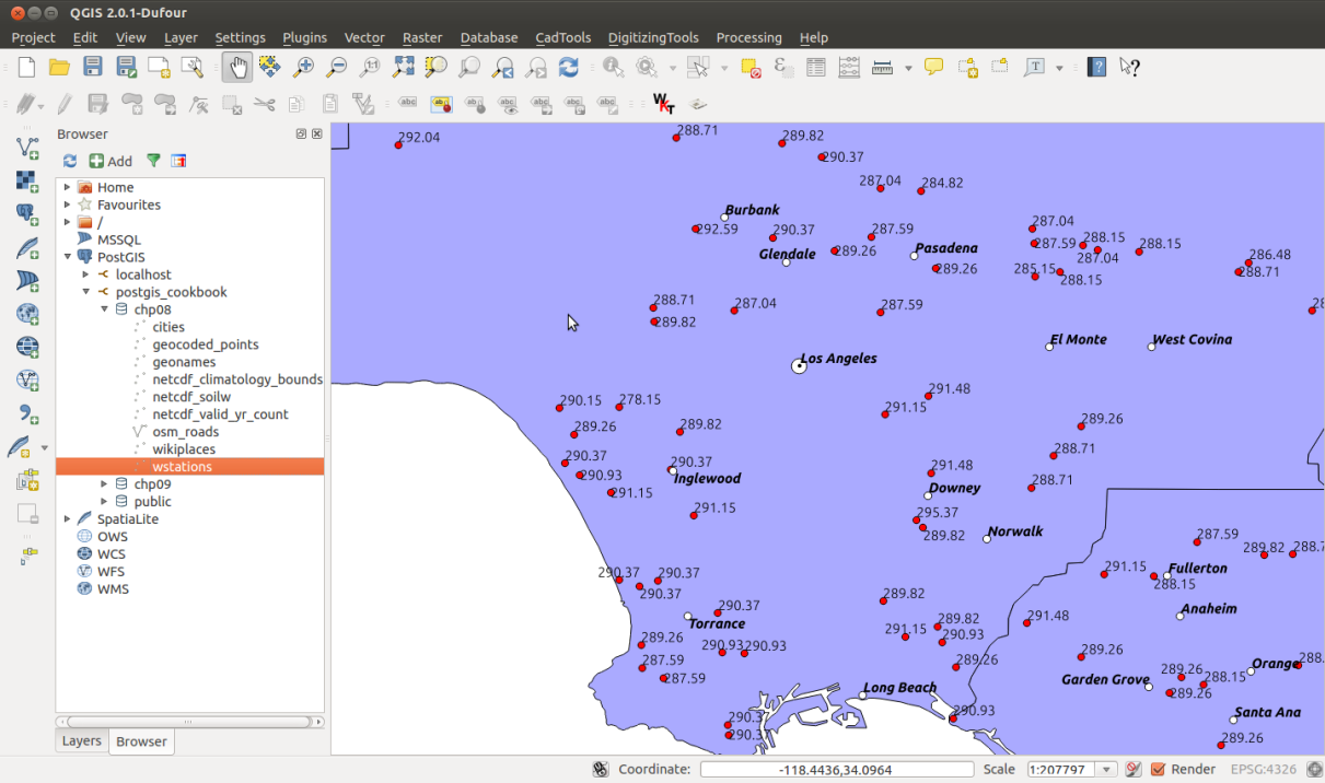
Psycopg is the most popular PostgreSQL adapter for Python, and it can be used to create Python scripts that send SQL commands to PostGIS. In this recipe, you created a Python script that queries weather data from the https://openweathermap.org/ web server using the popular JSON format to get the output data and then used that data to update two PostGIS layers.
For one of the layers, cities, the weather data is used to update the temperature field using the temperature data of the weather station closest to the city. For this purpose, you used an UPDATE SQL command. The other layer, wstations, is updated every time a new weather station is identified from the weather data and inserted in the layer. In this case, you used an INSERT SQL statement.
This is a quick overview of the script's behavior (you can find more details in the comments within the Python code). In the beginning, a PostgreSQL connection is created using the Psycopg connection object. The connection object is created using the main connection parameters (dbname, user, and password, while default values for server name and port are not specified; instead, localhost and 5432 are used). The connection behavior is set to auto commit so that any SQL performed by Psycopg will be run immediately and will not be embedded in a transaction.
Using a cursor, you first iterate all of the records in the cities PostGIS layer; for each of the cities, you need to get the temperature from the https://openweathermap.org/ web server. For this purpose, for each city you make a call to the GetWeatherData method, passing the coordinates of the city to it. The method queries the server using the requests library and parses the JSON response using the simplejson Python library.
You should send the URL request to a try...catch block. This way, if there is any issue with the web service (internet connection not available, or any HTTP status codes different from 200, or whatever else), the process can safely continue with the data of the next city (iteration).
The JSON response contains, as per the request, the information about the 10 weather stations closest to the city. You will use the information of the first weather station, the closest one to the city, to set the temperature field for the city.
You then iterate all of the station JSON objects, and by using the AddWeatherStation method, you create a weather station in the wstation PostGIS layer, but only if a weather station with the same id does not exist.
In this recipe, you will use Python and the Python bindings of the GDAL/OGR library to create a script for geocoding a list of the names of places using one of the GeoNames web services (http://www.geonames.org/export/ws-overview.html). You will use the Wikipedia Fulltext Search web service (http://www.geonames.org/export/wikipedia-webservice.html#wikipediaSearch), which for a given search string returns the coordinates of the places matching that search string as the output, and some other useful attributes from Wikipedia, including the Wikipedia page title and url.
The script should first create a PostGIS point layer named wikiplaces in which all of the locations and their attributes returned by the web service will be stored.
This recipe should give you the basis to use other similar web services, such as Google Maps, Yahoo! BOSS Geo Services, and so on, to get results in a similar way.
Before you start, please note the terms of use of GeoNames: http://www.geonames.org/export/. In a few words, at the time of writing, you have a 30,000 credits' daily limit per application (identified by the username parameter); the hourly limit is 2,000 credits. A credit is a web service request hit for most services.
You will generate the PostGIS table containing the geocoded place names using the GDAL/OGR Python bindings (http://trac.osgeo.org/gdal/wiki/GdalOgrInPython).
$ source postgis-cb-env/bin/activate
(postgis-cb-env)$ pip install gdal
(postgis-cb-env)$ pip install simplejson
Carry out the following steps:
You should get the following JSON output:
{
"geonames": [
{
"summary": "London is the capital and most populous city of
England and United Kingdom. Standing on the River Thames,
London has been a major settlement for two millennia,
its history going back to its founding by the Romans,
who named it Londinium (...)",
"elevation": 8,
"geoNameId": 2643743,
"feature": "city",
"lng": -0.11832,
"countryCode": "GB",
"rank": 100,
"thumbnailImg": "http://www.geonames.org/img/wikipedia/
43000/thumb-42715-100.jpg",
"lang": "en",
"title": "London",
"lat": 51.50939,
"wikipediaUrl": "en.wikipedia.org/wiki/London"
},
{
"summary": "New London is a city and a port of entry on the
northeast coast of the United States. It is located at
the mouth of the Thames River in New London County,
southeastern Connecticut. New London is located about from
the state capital of Hartford,
from Boston, Massachusetts, from Providence, Rhode (...)",
"elevation": 27,
"feature": "landmark",
"lng": -72.10083333333333,
"countryCode": "US",
"rank": 100,
"thumbnailImg": "http://www.geonames.org/img/wikipedia/
160000/thumb-159123-100.jpg",
"lang": "en",
"title": "New London, Connecticut",
"lat": 41.355555555555554,
"wikipediaUrl": "en.wikipedia.org/wiki/
New_London%2C_Connecticut"
},...
]
}
$ vi names.txt
London
Rome
Boston
Chicago
Madrid
Paris
...
import sys
import requests
import simplejson as json
from osgeo import ogr, osr
MAXROWS = 10
USERNAME = 'postgis' #enter your username here
def CreatePGLayer():
"""
Create the PostGIS table.
"""
driver = ogr.GetDriverByName('PostgreSQL')
srs = osr.SpatialReference()
srs.ImportFromEPSG(4326)
ogr.UseExceptions()
pg_ds = ogr.Open("PG:dbname='postgis_cookbook' host='localhost'
port='5432' user='me' password='password'", update = 1)
pg_layer = pg_ds.CreateLayer('wikiplaces', srs = srs,
geom_type=ogr.wkbPoint, options = [
'DIM=3',
# we want to store the elevation value in point z coordinate
'GEOMETRY_NAME=the_geom',
'OVERWRITE=YES',
# this will drop and recreate the table every time
'SCHEMA=chp08',
])
# add the fields
fd_title = ogr.FieldDefn('title', ogr.OFTString)
pg_layer.CreateField(fd_title)
fd_countrycode = ogr.FieldDefn('countrycode', ogr.OFTString)
pg_layer.CreateField(fd_countrycode)
fd_feature = ogr.FieldDefn('feature', ogr.OFTString)
pg_layer.CreateField(fd_feature)
fd_thumbnail = ogr.FieldDefn('thumbnail', ogr.OFTString)
pg_layer.CreateField(fd_thumbnail)
fd_wikipediaurl = ogr.FieldDefn('wikipediaurl', ogr.OFTString)
pg_layer.CreateField(fd_wikipediaurl)
return pg_ds, pg_layer
def AddPlacesToLayer(places):
"""
Read the places dictionary list and add features in the
PostGIS table for each place.
"""
# iterate every place dictionary in the list
print "places: ", places
for place in places:
lng = place['lng']
lat = place['lat']
z = place.get('elevation') if 'elevation' in place else 0
# we generate a point representation in wkt,
# and create an ogr geometry
point_wkt = 'POINT(%s %s %s)' % (lng, lat, z)
point = ogr.CreateGeometryFromWkt(point_wkt)
# we create a LayerDefn for the feature using the one
# from the layer
featureDefn = pg_layer.GetLayerDefn()
feature = ogr.Feature(featureDefn)
# now time to assign the geometry and all the
# other feature's fields, if the keys are contained
# in the dictionary (not always the GeoNames
# Wikipedia Fulltext Search contains all of the information)
feature.SetGeometry(point)
feature.SetField('title',
place['title'].encode("utf-8") if 'title' in place else '')
feature.SetField('countrycode',
place['countryCode'] if 'countryCode' in place else '')
feature.SetField('feature',
place['feature'] if 'feature' in place else '')
feature.SetField('thumbnail',
place['thumbnailImg'] if 'thumbnailImg' in place else '')
feature.SetField('wikipediaurl',
place['wikipediaUrl'] if 'wikipediaUrl' in place else '')
# here we create the feature (the INSERT SQL is issued here)
pg_layer.CreateFeature(feature)
print 'Created a places titled %s.' % place['title']
def GetPlaces(placename):
"""
Get the places list for a given placename.
"""
# uri to access the JSON GeoNames Wikipedia Fulltext Search
# web service
uri = ('http://api.geonames.org/wikipediaSearchJSON?
formatted=true&q=%s&maxRows=%s&username=%s&style=full'
% (placename, MAXROWS, USERNAME))
data = requests.get(uri)
js_data = json.loads(data.text)
return js_data['geonames']
def GetNamesList(filepath):
"""
Open a file with a given filepath containing place names
and return a list.
"""
f = open(filepath, 'r')
return f.read().splitlines()
# first we need to create a PostGIS table to contains the places
# we must keep the PostGIS OGR dataset and layer global,
# for the reasons
# described here: http://trac.osgeo.org/gdal/wiki/PythonGotchas
from osgeo import gdal
gdal.UseExceptions()
pg_ds, pg_layer = CreatePGLayer()
try:
# query geonames for each name and store found
# places in the table
names = GetNamesList('names.txt')
print names
for name in names:
AddPlacesToLayer(GetPlaces(name))
except Exception as e:
print(e)
print sys.exc_info()[0]
(postgis-cb-env)$ python import_places.py
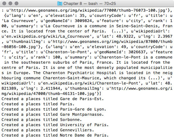
postgis_cookbook=# select ST_AsText(the_geom), title,
countrycode, feature from chp08.wikiplaces;
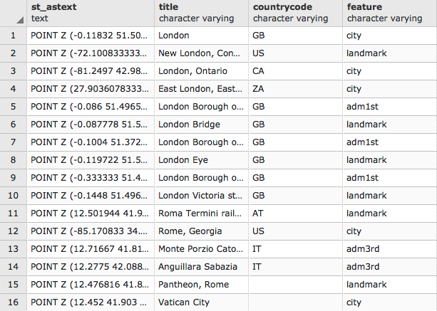
(60 rows)
This Python script uses the requests and simplejson libraries to fetch data from the GeoNames wikipediaSearchJSON web service, and the GDAL/OGR library to store geographic information inside the PostGIS database.
First, you create a PostGIS point table to store the geographic data. This is made using the GDAL/OGR bindings. You need to instantiate an OGR PostGIS driver (http://www.gdal.org/drv_pg.html) from where it is possible to instantiate a dataset to connect to your postgis_cookbook database using a specified connection string.
The update parameter in the connection string specifies to the GDAL driver that you will open the dataset for updating.
From the PostGIS dataset, we created a PostGIS layer named wikiplaces that will store points (geom_type=ogr.wkbPoint) using the WGS 84 spatial reference system (srs.ImportFromEPSG(4326)). When creating the layer, we specified other parameters as well, such as dimension (3, as you want to store the z values), GEOMETRY_NAME (name of the geometric field), and schema. After creating the layer, you can use the CreateField layer method to create all the fields that are needed to store the information. Each field will have a specific name and datatype (all of them are ogr.OFTString in this case).
After the layer has been created (note that we need to have the pg_ds and pg_layer objects always in context for the whole script, as noted at http://trac.osgeo.org/gdal/wiki/PythonGotchas), you can query the GeoNames web services for each place name in the names.txt file using the urllib2 library.
We parsed the JSON response using the simplejson library, then iterated the JSON objects list and added a feature to the PostGIS layer for each of the objects in the JSON output. For each element, we created a feature with a point wkt geometry (using the lng, lat, and elevation object attributes) using the ogr.CreateGeometryFromWkt method, and updated the other fields using the other object attributes returned by GeoNames, using the feature setField method (title, countryCode, and so on).
You can get more information on programming with GDAL Python bindings by using the following great resource by Chris Garrard:
In this recipe, you will write a Python function for PostGIS using the PL/Python language. The PL/Python procedural language allows you to write PostgreSQL functions with the Python language.
You will use Python to query the http://openweathermap.org/ web services, already used in a previous recipe, to get the weather for a PostGIS geometry from within a PostgreSQL function.
$ sudo apt-get install postgresql-plpython-9.1
Carry out the following steps:
{
message: "",
cod: "200",
calctime: "",
cnt: 1,
list: [
{
id: 9191,
dt: 1369343192,
name: "100704-1",
type: 2,
coord: {
lat: 13.7408,
lon: 100.5478
},
distance: 6.244,
main: {
temp: 300.37
},
wind: {
speed: 0,
deg: 141
},
rang: 30,
rain: {
1h: 0,
24h: 3.302,
today: 0
}
}
]
}
CREATE OR REPLACE FUNCTION chp08.GetWeather(lon float, lat float)
RETURNS float AS $$
import urllib2
import simplejson as json
data = urllib2.urlopen(
'http://api.openweathermap.org/data/
2.1/find/station?lat=%s&lon=%s&cnt=1'
% (lat, lon))
js_data = json.load(data)
if js_data['cod'] == '200':
# only if cod is 200 we got some effective results
if int(js_data['cnt'])>0:
# check if we have at least a weather station
station = js_data['list'][0]
print 'Data from weather station %s' % station['name']
if 'main' in station:
if 'temp' in station['main']:
temperature = station['main']['temp'] - 273.15
# we want the temperature in Celsius
else:
temperature = None
else:
temperature = None
return temperature $$ LANGUAGE plpythonu;
postgis_cookbook=# SELECT chp08.GetWeather(100.49, 13.74);
getweather ------------ 27.22 (1 row)
postgis_cookbook=# SELECT name, temperature,
chp08.GetWeather(ST_X(the_geom), ST_Y(the_geom))
AS temperature2 FROM chp08.cities LIMIT 5; name | temperature | temperature2 -------------+-------------+-------------- Minneapolis | 275.15 | 15 Saint Paul | 274.15 | 16 Buffalo | 274.15 | 19.44 New York | 280.93 | 19.44 Jersey City | 282.15 | 21.67 (5 rows)
CREATE OR REPLACE FUNCTION chp08.GetWeather(geom geometry)
RETURNS float AS $$ BEGIN RETURN chp08.GetWeather(ST_X(ST_Centroid(geom)),
ST_Y(ST_Centroid(geom)));
END;
$$ LANGUAGE plpgsql;
postgis_cookbook=# SELECT chp08.GetWeather(
ST_GeomFromText('POINT(-71.064544 42.28787)')); getweather ------------ 23.89 (1 row)
postgis_cookbook=# SELECT name, temperature,
chp08.GetWeather(the_geom) AS temperature2
FROM chp08.cities LIMIT 5; name | temperature | temperature2 -------------+-------------+-------------- Minneapolis | 275.15 | 17.22 Saint Paul | 274.15 | 16 Buffalo | 274.15 | 18.89 New York | 280.93 | 19.44 Jersey City | 282.15 | 21.67 (5 rows)
In this recipe, you wrote a Python function in PostGIS, using the PL/Python language. Using Python inside PostgreSQL and PostGIS functions gives you the great advantage of being able to use any Python library you wish. Therefore, you will be able to write much more powerful functions compared to those written using the standard PL/PostgreSQL language.
In fact, in this case, you used the urllib2 and simplejson Python libraries to query a web service from within a PostgreSQL function—this would be an impossible operation to do using plain PL/PostgreSQL. You have also seen how to overload functions in order to provide the function's user a different way to access the function, using input parameters in a different way.
In this recipe, you will write two PL/PostgreSQL PostGIS functions that will let you perform geocoding and reverse geocoding using the GeoNames datasets.
GeoNames is a database of place names in the world, containing over 8 million records that are available for download free of charge. For the purpose of this recipe, you will download a part of the database, load it in PostGIS, and then use it within two functions to perform geocoding and reverse geocoding. Geocoding is the process of finding coordinates from geographical data, such as an address or a place name, while reverse geocoding is the process of finding geographical data, such as an address or place name, from its coordinates.
You are going to write the two functions using PL/pgSQL, which adds on top of the PostgreSQL SQL commands the ability to tie more commands and queries together, a bunch of control structures, cursors, error management, and other goodness.
Download a GeoNames dataset. At the time of writing, you can find some of the datasets ready to be downloaded from http://download.geonames.org/export/dump/. You may decide which dataset you want to use; if you want to follow this recipe, it will be enough to download the Italian dataset, IT.zip (included in the book's dataset, in the chp08 directory).
If you want to download the full GeoNames dataset, you need to download the allCountries.zip file; it will take longer as it is about 250 MB.
Carry out the following steps:
geonameid : integer id of record in geonames database
name : name of geographical point (utf8) varchar(200)
asciiname : name of geographical point in plain
ascii characters, varchar(200)
alternatenames : alternatenames, comma separated varchar(5000)
latitude : latitude in decimal degrees (wgs84)
longitude : longitude in decimal degrees (wgs84)
...
$ ogrinfo CSV:IT.txt IT -al -so
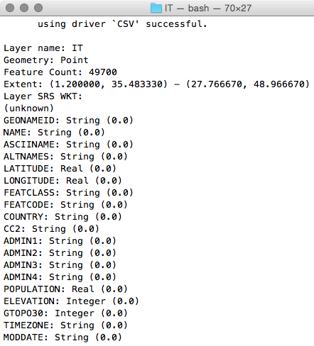
$ ogrinfo CSV:IT.txt IT -where "NAME = 'San Gimignano'"
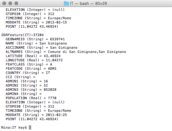
$ ogr2ogr -f PostgreSQL -s_srs EPSG:4326 -t_srs EPSG:4326
-lco GEOMETRY_NAME=the_geom -nln chp08.geonames
PG:"dbname='postgis_cookbook' user='me' password='mypassword'"
CSV:IT.txt -sql "SELECT NAME, ASCIINAME FROM IT"
postgis_cookbook=# SELECT ST_AsText(the_geom), name
FROM chp08.geonames LIMIT 10;
CREATE OR REPLACE FUNCTION chp08.Get_Closest_PlaceNames(
in_geom geometry, num_results int DEFAULT 5,
OUT geom geometry, OUT place_name character varying)
RETURNS SETOF RECORD AS $$
BEGIN
RETURN QUERY
SELECT the_geom as geom, name as place_name
FROM chp08.geonames
ORDER BY the_geom <-> ST_Centroid(in_geom) LIMIT num_results;
END; $$ LANGUAGE plpgsql;
postgis_cookbook=# SELECT * FROM chp08.Get_Closest_PlaceNames(
ST_PointFromText('POINT(13.5 42.19)', 4326), 10);
The following is the output for this query:
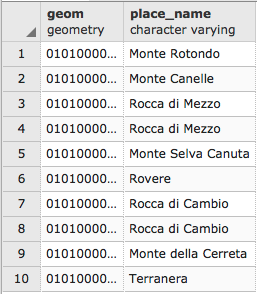
postgis_cookbook=# SELECT * FROM chp08.Get_Closest_PlaceNames(
ST_PointFromText('POINT(13.5 42.19)', 4326));
And you will get the following rows:
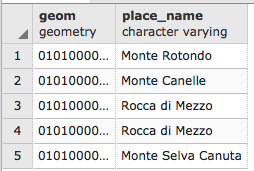
CREATE OR REPLACE FUNCTION chp08.Find_PlaceNames(search_string text,
num_results int DEFAULT 5,
OUT geom geometry,
OUT place_name character varying)
RETURNS SETOF RECORD AS $$
BEGIN
RETURN QUERY
SELECT the_geom as geom, name as place_name
FROM chp08.geonames
WHERE name @@ to_tsquery(search_string)
LIMIT num_results;
END; $$ LANGUAGE plpgsql;
postgis_cookbook=# SELECT * FROM chp08.Find_PlaceNames('Rocca', 10);
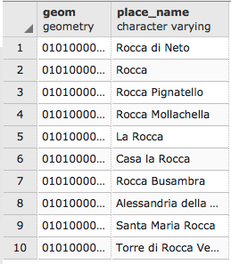
In this recipe, you wrote two PostgreSQL functions to perform geocoding and reverse geocoding. For both the functions, you defined a set of input and output parameters, and after some PL/PostgreSQL processing, you returned a set of records to the function client, given by executing a query.
As the input parameters, the Get_Closest_PlaceNames function accepts a PostGIS geometry and an optional num_results parameter that is set to a default of 5 in case the function caller does not provide it. The output of this function is SETOF RECORD, which is returned after running a query in the function body (defined by the $$ notation). Here, the query finds the places closest to the centroid of the input geometry. This is done using an indexed nearest neighbor search (KNN index), a new feature available in PostGIS 2.
The Find_PlaceNames function accepts as the input parameters a search string to look for and an optional num_results parameter, which in this case is also set to a default of 5 if not provided by the function caller. The output is a SETOF RECORD, which is returned after running a query that uses the to_tsquery PostgreSQL text search function. The results of the query are the places from the database that contain the search_string value in the name field.
In this recipe, you will use OpenStreetMap streets' datasets imported in PostGIS to implement a very basic Python class in order to provide geocoding features to the class' consumer. The geocode engine will be based on the implementation of the PostgreSQL trigrams provided by the contrib module of PostgreSQL: pg_trgm.
A trigram is a group of three consecutive characters contained in a string, and it is a very effective way to measure the similarity of two strings by counting the number of trigrams they have in common.
This recipe aims to be a very basic sample to implement some kinds of geocoding functionalities (it will just return one or more points from a street name), but it could be extended to support more advanced features.
$ ogrinfo --version GDAL 2.1.2, released 2016/10/24
$ ogrinfo --formats | grep -i osm
-> "OSM -vector- (rov): OpenStreetMap XML and PBF"
$ sudo apt-get install postgresql-contrib-9.1
postgis_cookbook=# CREATE EXTENSION pg_trgm;
CREATE EXTENSION
You will need to use some OSM datasets included in the source for this chapter. (in the data/chp08 book's dataset directory). If you are using Windows, be sure to have installed the OSGeo4W suite, as suggested in the initial instructions for this chapter.
$ source postgis-cb-env/bin/activate
(postgis-cb-env)$ pip install pygdal
(postgis-cb-env)$ pip install psycopg2
Carry out the following steps:
$ ogrinfo lazio.pbf
Had to open data source read-only.
INFO: Open of `lazio.pbf'
using driver `OSM' successful.
1: points (Point)
2: lines (Line String)
3: multilinestrings (Multi Line String)
4: multipolygons (Multi Polygon) 5: other_relations (Geometry Collection)
$ ogr2ogr -f PostgreSQL -lco GEOMETRY_NAME=the_geom
-nln chp08.osm_roads
PG:"dbname='postgis_cookbook' user='me'
password='mypassword'" lazio.pbf lines
postgis_cookbook=# SELECT name,
similarity(name, 'via benedetto croce') AS sml,
ST_AsText(ST_Centroid(the_geom)) AS the_geom
FROM chp08.osm_roads
WHERE name % 'via benedetto croce'
ORDER BY sml DESC, name;
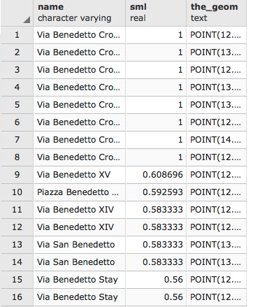
postgis_cookbook=# SELECT name,
name <-> 'via benedetto croce' AS weight
FROM chp08.osm_roads
ORDER BY weight LIMIT 10;
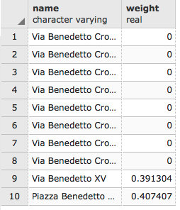
import sys
import psycopg2
class OSMGeocoder(object):
"""
A class to provide geocoding features using an OSM
dataset in PostGIS.
"""
def __init__(self, db_connectionstring):
# initialize db connection parameters
self.db_connectionstring = db_connectionstring
def geocode(self, placename):
"""
Geocode a given place name.
"""
# here we create the connection object
conn = psycopg2.connect(self.db_connectionstring)
cur = conn.cursor()
# this is the core sql query, using trigrams to detect
# streets similar to a given placename
sql = """
SELECT name, name <-> '%s' AS weight,
ST_AsText(ST_Centroid(the_geom)) as point
FROM chp08.osm_roads
ORDER BY weight LIMIT 10;
""" % placename
# here we execute the sql and return all of the results
cur.execute(sql)
rows = cur.fetchall()
cur.close()
conn.close()
return rows
if __name__ == '__main__':
# the user must provide at least two parameters, the place name
# and the connection string to PostGIS
if len(sys.argv) < 3 or len(sys.argv) > 3:
print "usage: <placename> <connection string>"
raise SystemExit
placename = sys.argv[1]
db_connectionstring = sys.argv[2]
# here we instantiate the geocoder, providing the needed
# PostGIS connection parameters
geocoder = OSMGeocoder(db_connectionstring)
# here we query the geocode method, for getting the
# geocoded points for the given placename
results = geocoder.geocode(placename)
print results
(postgis-cb-env)$ python osmgeocoder.py "Via Benedetto Croce"
"dbname=postgis_cookbook user=me password=mypassword"
[('Via Benedetto Croce', 0.0, 'POINT(12.6999095325807
42.058016054317)'),...
Via Delle Sette Chiese
Via Benedetto Croce
Lungotevere Degli Inventori
Viale Marco Polo Via Cavour
from osmgeocoder import OSMGeocoder
from osgeo import ogr, osr
# here we read the file
f = open('streets.txt')
streets = f.read().splitlines()
f.close()
# here we create the PostGIS layer using gdal/ogr
driver = ogr.GetDriverByName('PostgreSQL')
srs = osr.SpatialReference()
srs.ImportFromEPSG(4326)
pg_ds = ogr.Open(
"PG:dbname='postgis_cookbook' host='localhost' port='5432'
user='me' password='mypassword'", update = 1 )
pg_layer = pg_ds.CreateLayer('geocoded_points', srs = srs,
geom_type=ogr.wkbPoint, options = [
'GEOMETRY_NAME=the_geom',
'OVERWRITE=YES',
# this will drop and recreate the table every time
'SCHEMA=chp08',
])
# here we add the field to the PostGIS layer
fd_name = ogr.FieldDefn('name', ogr.OFTString)
pg_layer.CreateField(fd_name)
print 'Table created.'
# now we geocode all of the streets in the file
# using the osmgeocoder class
geocoder = OSMGeocoder('dbname=postgis_cookbook user=me
password=mypassword')
for street in streets:
print street
geocoded_street = geocoder.geocode(street)[0]
print geocoded_street
# format is
# ('Via delle Sette Chiese', 0.0,
# 'POINT(12.5002166330412 41.859774874774)')
point_wkt = geocoded_street[2]
point = ogr.CreateGeometryFromWkt(point_wkt)
# we create a LayerDefn for the feature using the
# one from the layer
featureDefn = pg_layer.GetLayerDefn()
feature = ogr.Feature(featureDefn)
# now we store the feature geometry and
# the value for the name field
feature.SetGeometry(point)
feature.SetField('name', geocoded_street[0])
# finally we create the feature
# (an INSERT command is issued only here) pg_layer.CreateFeature(feature)
(postgis-cb-env)capooti@ubuntu:~/postgis_cookbook/working/chp08$
python geocode_streets.py
Table created.
Via Delle Sette Chiese
('Via delle Sette Chiese', 0.0,
'POINT(12.5002166330412 41.859774874774)')
...
Via Cavour ('Via Cavour', 0.0, 'POINT(12.7519263341222 41.9631244835521)')
For this recipe, you first imported an OSM dataset to PostGIS with ogr2ogr, using the GDAL OSM driver.
Then, you created a Python class, OSMGeocoder, to provide very basic support to the class consumer for geocoding street names, using the OSM data imported in PostGIS. For this purpose, you used the trigram support included in PostgreSQL with the pg_trgm contrib module.
The class that you have written is mainly composed of two methods: the __init__ method, where the connection parameters must be passed in order to instantiate an OSMGeocoder object, and the geocode method. The geocode method accepts an input parameter, placename, and creates a connection to the PostGIS database using the Psycopg2 library in order to execute a query to find the streets in the database with a name similar to the placename parameter.
The class can be consumed both from the command line, using the __name__ == '__main__' code block, or from an external Python code. You tried both approaches. In the latter, you created another Python script, where you imported the OSMGeocoder class combined with the GDAL/OGR Python bindings to generate a new PostGIS point layer with features resulted from a list of geocoded street names.
In this recipe, you will geocode addresses using web geocoding APIs, such as Google Maps, Yahoo! Maps, Geocoder, GeoNames, and so on. Be sure to read the terms of service of these APIs carefully before using them in production.
The geopy Python library (https://github.com/geopy/geopy) offers convenient uniform access to all of these web services. Therefore, you will use it to create a PL/Python PostgreSQL function that can be used in your SQL commands to query all of these engines.
In a Debian/Ubuntu box, it is as easy as typing the following:
$ sudo pip install geopy
In Windows, you can use the following command:
> pip install geopy
$ sudo apt-get install postgresql-plpython-9.1
$ psql -U me postgis_cookbook
psql (9.1.6, server 9.1.8)
Type "help" for help. postgis_cookbook=# CREATE EXTENSION plpythonu;
Carry out the following steps:
CREATE OR REPLACE FUNCTION chp08.Geocode(address text)
RETURNS geometry(Point,4326) AS $$
from geopy import geocoders
g = geocoders.GoogleV3()
place, (lat, lng) = g.geocode(address)
plpy.info('Geocoded %s for the address: %s' % (place, address))
plpy.info('Longitude is %s, Latitude is %s.' % (lng, lat))
plpy.info("SELECT ST_GeomFromText('POINT(%s %s)', 4326)"
% (lng, lat))
result = plpy.execute("SELECT ST_GeomFromText('POINT(%s %s)',
4326) AS point_geocoded" % (lng, lat))
geometry = result[0]["point_geocoded"]
return geometry $$ LANGUAGE plpythonu;
postgis_cookbook=# SELECT chp08.Geocode('Viale Ostiense 36, Rome');
INFO: Geocoded Via Ostiense, 36, 00154 Rome,
Italy for the address: Viale Ostiense 36, Rome
CONTEXT: PL/Python function "geocode"
INFO: Longitude is 12.480457, Latitude is 41.874345.
CONTEXT: PL/Python function "geocode"
INFO: SELECT ST_GeomFromText('POINT(12.480457 41.874345)', 4326)
CONTEXT: PL/Python function "geocode"
geocode
----------------------------------------------------
0101000020E6100000BF44BC75FEF52840E7357689EAEF4440
(1 row)
CREATE OR REPLACE FUNCTION chp08.Geocode(address text,
api text DEFAULT 'google')
RETURNS geometry(Point,4326) AS $$
from geopy import geocoders
plpy.info('Geocoing the given address using the %s api' % (api))
if api.lower() == 'geonames':
g = geocoders.GeoNames()
elif api.lower() == 'geocoderdotus':
g = geocoders.GeocoderDotUS()
else: # in all other cases, we use google
g = geocoders.GoogleV3()
try:
place, (lat, lng) = g.geocode(address)
plpy.info('Geocoded %s for the address: %s' % (place, address))
plpy.info('Longitude is %s, Latitude is %s.' % (lng, lat))
result = plpy.execute("SELECT ST_GeomFromText('POINT(%s %s)',
4326) AS point_geocoded" % (lng, lat))
geometry = result[0]["point_geocoded"]
return geometry
except:
plpy.warning('There was an error in the geocoding process,
setting geometry to Null.')
return None $$ LANGUAGE plpythonu;
postgis_cookbook=# SELECT chp08.Geocode('161 Court Street,
Brooklyn, NY');
INFO: Geocoing the given address using the google api
CONTEXT: PL/Python function "geocode2"
INFO: Geocoded 161 Court Street, Brooklyn, NY 11201,
USA for the address: 161 Court Street, Brooklyn, NY
CONTEXT: PL/Python function "geocode2"
INFO: Longitude is -73.9924659, Latitude is 40.688665.
CONTEXT: PL/Python function "geocode2"
INFO: SELECT ST_GeomFromText('POINT(-73.9924659 40.688665)', 4326)
CONTEXT: PL/Python function "geocode2"
geocode2
----------------------------------------------------
0101000020E61000004BB9B18F847F52C02E73BA2C26584440
(1 row)
postgis_cookbook=# SELECT chp08.Geocode('161 Court Street,
Brooklyn, NY', 'GeocoderDotUS');
INFO: Geocoing the given address using the GeocoderDotUS api
CONTEXT: PL/Python function "geocode2"
INFO: Geocoded 161 Court St, New York, NY 11201 for the address: 161
Court Street, Brooklyn, NY
CONTEXT: PL/Python function "geocode2"
INFO: Longitude is -73.992809, Latitude is 40.688774.
CONTEXT: PL/Python function "geocode2"
INFO: SELECT ST_GeomFromText('POINT(-73.992809 40.688774)', 4326)
CONTEXT: PL/Python function "geocode2"
geocode2
----------------------------------------------------
0101000020E61000002A8BC22E8A7F52C0E52A16BF29584440
(1 row)
You wrote a PL/Python function to geocode an address. For this purpose, you used the geopy Python library, which lets you query several geocoding APIs in the same manner.
Using geopy, you need to instantiate a geocoder object with a given API and query it to get the results, such as a place name and a couple of coordinates. You can use the plpy module utilities to run a query on the database using the PostGIS ST_GeomFromText function, and log informative messages and warnings for the user.
If the geocoding process fails, you return a NULL geometry to the user with a warning message, using a try..except Python block.
In this recipe, you will write a Python script to import data from the NetCDF format to PostGIS.
NetCDF is an open standard format, widely used for scientific applications, and can contain multiple raster datasets, each composed of a spectrum of bands. For this purpose, you will use the GDAL Python bindings and the popular NumPy (http://www.numpy.org/) scientific library.
For Linux users, in case you did not do it yet, follow the initial instructions for this chapter and create a Python virtual environment in order to keep a Python-isolated environment to be used for all the Python recipes in this book. Then, activate it:
$ source postgis-cb-env/bin/activate
(postgis-cb-env)$ pip uninstall gdal
(postgis-cb-env)$ pip install numpy (postgis-cb-env)$ pip install gdal
Carry out the following steps:
$ gdalinfo NETCDF:"soilw.mon.ltm.v2.nc"
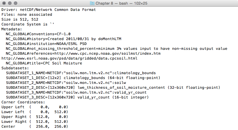
$ gdalinfo NETCDF:"soilw.mon.ltm.v2.nc":soilw
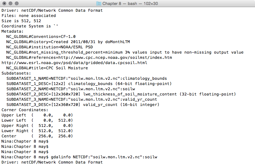 '
'...(12 bands)...
import sys
from osgeo import gdal, ogr, osr
from osgeo.gdalconst import GA_ReadOnly, GA_Update
def netcdf2postgis(file_nc, pg_connection_string,
postgis_table_prefix):
# register gdal drivers
gdal.AllRegister()
# postgis driver, needed to create the tables
driver = ogr.GetDriverByName('PostgreSQL')
srs = osr.SpatialReference()
# for simplicity we will assume all of the bands in the datasets
# are in the same spatial reference, wgs 84
srs.ImportFromEPSG(4326)
# first, check if dataset exists
ds = gdal.Open(file_nc, GA_ReadOnly)
if ds is None:
print 'Cannot open ' + file_nc
sys.exit(1)
# 1. iterate subdatasets
for sds in ds.GetSubDatasets():
dataset_name = sds[0]
variable = sds[0].split(':')[-1]
print 'Importing from %s the variable %s...' %
(dataset_name, variable)
# open subdataset and read its properties
sds = gdal.Open(dataset_name, GA_ReadOnly)
cols = sds.RasterXSize
rows = sds.RasterYSize
bands = sds.RasterCount
# create a PostGIS table for the subdataset variable
table_name = '%s_%s' % (postgis_table_prefix, variable)
pg_ds = ogr.Open(pg_connection_string, GA_Update )
pg_layer = pg_ds.CreateLayer(table_name, srs = srs,
geom_type=ogr.wkbPoint, options = [
'GEOMETRY_NAME=the_geom',
'OVERWRITE=YES',
# this will drop and recreate the table every time
'SCHEMA=chp08',
])
print 'Table %s created.' % table_name
# get georeference transformation information
transform = sds.GetGeoTransform()
pixelWidth = transform[1]
pixelHeight = transform[5]
xOrigin = transform[0] + (pixelWidth/2)
yOrigin = transform[3] - (pixelWidth/2)
# 2. iterate subdataset bands and append them to data
data = []
for b in range(1, bands+1):
band = sds.GetRasterBand(b)
band_data = band.ReadAsArray(0, 0, cols, rows)
data.append(band_data)
# here we add the fields to the table, a field for each band
# check datatype (Float32, 'Float64', ...)
datatype = gdal.GetDataTypeName(band.DataType)
ogr_ft = ogr.OFTString # default for a field is string
if datatype in ('Float32', 'Float64'):
ogr_ft = ogr.OFTReal
elif datatype in ('Int16', 'Int32'):
ogr_ft = ogr.OFTInteger
# here we add the field to the PostGIS layer
fd_band = ogr.FieldDefn('band_%s' % b, ogr_ft)
pg_layer.CreateField(fd_band)
print 'Field band_%s created.' % b
# 3. iterate rows and cols
for r in range(0, rows):
y = yOrigin + (r * pixelHeight)
for c in range(0, cols):
x = xOrigin + (c * pixelWidth)
# for each cell, let's add a point feature
# in the PostGIS table
point_wkt = 'POINT(%s %s)' % (x, y)
point = ogr.CreateGeometryFromWkt(point_wkt)
featureDefn = pg_layer.GetLayerDefn()
feature = ogr.Feature(featureDefn)
# now iterate bands, and add a value for each table's field
for b in range(1, bands+1):
band = sds.GetRasterBand(1)
datatype = gdal.GetDataTypeName(band.DataType)
value = data[b-1][r,c]
print 'Storing a value for variable %s in point x: %s,
y: %s, band: %s, value: %s' % (variable, x, y, b, value)
if datatype in ('Float32', 'Float64'):
value = float(data[b-1][r,c])
elif datatype in ('Int16', 'Int32'):
value = int(data[b-1][r,c])
else:
value = data[r,c]
feature.SetField('band_%s' % b, value)
# set the feature's geometry and finalize its creation
feature.SetGeometry(point) pg_layer.CreateFeature(feature)
if __name__ == '__main__':
# the user must provide at least three parameters,
# the netCDF file path, the PostGIS GDAL connection string # and the prefix suffix to use for PostGIS table names
if len(sys.argv) < 4 or len(sys.argv) > 4:
print "usage: <netCDF file path> <GDAL PostGIS connection
string><PostGIS table prefix>"
raise SystemExit
file_nc = sys.argv[1]
pg_connection_string = sys.argv[2]
postgis_table_prefix = sys.argv[3] netcdf2postgis(file_nc, pg_connection_string,
postgis_table_prefix)
(postgis-cb-env)$ python netcdf2postgis.py
NETCDF:"soilw.mon.ltm.v2.nc"
"PG:dbname='postgis_cookbook' host='localhost'
port='5432' user='me' password='mypassword'" netcdf
Importing from NETCDF:"soilw.mon.ltm.v2.nc":
climatology_bounds the variable climatology_bounds...
...
Importing from NETCDF:"soilw.mon.ltm.v2.nc":soilw the
variable soilw...
Table netcdf_soilw created.
Field band_1 created.
Field band_2 created.
...
Field band_11 created.
Field band_12 created.
Storing a value for variable soilw in point x: 0.25,
y: 89.75, band: 2, value: -9.96921e+36
Storing a value for variable soilw in point x: 0.25,
y: 89.75, band: 3, value: -9.96921e+36 ...
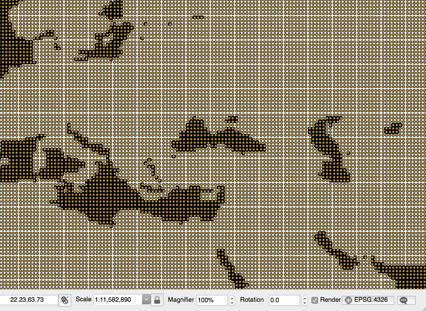
You have used Python with GDAL and NumPy in order to create a command-line utility to import a NetCDF dataset into PostGIS.
A NetCDF dataset is composed of multiple subdatasets, and each subdataset is composed of multiple raster bands. Each band is composed of cells. This structure should be clear to you after investigating a sample NetCDF dataset using the gdalinfo GDAL command tool.
There are several approaches to exporting cell values to PostGIS. The approach you adopted here is to generate a PostGIS point layer for each subdataset, which is composed of one field for each subdataset band. You then iterated the raster cells and appended a point to the PostGIS layer with the values read from each cell band.
The way you do this with Python is by using the GDAL Python bindings. For reading, you open the NetCDF dataset, and for updating, you open the PostGIS database, using the correct GDAL and OGR drivers. Then, you iterate the NetCDF subdatasets, using the GetSubDatasets method, and create a PostGIS table named NetCDF subdataset variable (with the prefix) for each subdataset, using the CreateLayer method.
For each subdataset, you iterate its bands, using the GetRasterBand method. To read each band, you run the ReadAsArray method which uses NumPy to get the band as an array.
For each band, you create a field in the PostGIS layer with the correct field data type that will be able to store the band's values. To choose the correct data type, you investigate the band's data type, using the DataType property.
Finally, you iterate the raster cells, by reading the correct x and y coordinates using the subdataset transform parameters, available via the GetGeoTransform method. For each cell, you create a point with the CreateGeometryFromWkt method, then set the field values, and read from the band array using the SetField feature method.
Finally, you append the new point to the PostGIS layer using the CreateFeature method.
In this chapter, we will cover the following topics:
In this chapter, we will try to give you an overview of how you can use PostGIS to develop powerful GIS web applications, using Open Geospatial Consortium (OGC) web standards such as Web Map Service (WMS) and Web Feature Service (WFS).
In the first two recipes, you will get an overview of two very popular open source web-mapping engines, MapServer and GeoServer. In both these recipes, you will see how to implement WMS and WFS services using PostGIS layers.
In the third recipe, you will implement a WMS Time service using MapServer to expose time-series data.
In the next two recipes, you will learn how to consume these web services to create web map viewers with two very popular JavaScript clients. In the fourth recipe, you will use a WMS service with OpenLayers, while in the fifth recipe, you will do the same thing using Leaflet.
In the sixth recipe, you will explore the power of transactional WFS to create web-mapping applications to enable editing data.
In the next two recipes, you will unleash the power of the popular Django web framework, which is based on Python, and its nice GeoDjango library, and see how it is possible to implement a powerful CRUD GIS web application. In the seventh recipe, you will create the back office for this application using the Django Admin site, and in the last recipe of the chapter, you will develop a frontend for users to display data from the application in a web map based on Leaflet.
Finally, in the last recipe, you will learn how to import your PostGIS data into Mapbox using OGR to create a custom web GPX viewer.
In this recipe, you will see how to create a WMS and WFS from a PostGIS layer, using the popular MapServer open source web-mapping engine.
You will then use the services, testing their exposed requests, using first a browser and then a desktop tool such as QGIS (you could do this using other software, such as uDig, gvSIG, and OpenJUMP GIS).
Follow these steps before getting ready:
postgis_cookbook=# create schema chp09;
On Linux, run the $ /usr/lib/cgi-bin/mapserv -v command and check for the following output:
MapServer version 7.0.7 OUTPUT=GIF OUTPUT=PNG OUTPUT=JPEG SUPPORTS=PROJ
SUPPORTS=GD SUPPORTS=AGG SUPPORTS=FREETYPE SUPPORTS=CAIRO
SUPPORTS=SVG_SYMBOLS
SUPPORTS=ICONV SUPPORTS=FRIBIDI SUPPORTS=WMS_SERVER SUPPORTS=WMS_CLIENT
SUPPORTS=WFS_SERVER SUPPORTS=WFS_CLIENT SUPPORTS=WCS_SERVER
SUPPORTS=SOS_SERVER SUPPORTS=FASTCGI SUPPORTS=THREADS SUPPORTS=GEOS
INPUT=JPEG INPUT=POSTGIS INPUT=OGR INPUT=GDAL INPUT=SHAPEFILE
On Windows, run the following command:
c:\ms4w\Apache\cgi-bin\mapserv.exe -v
On macOS, use the $ mapserv -v command:
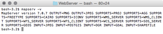
$ shp2pgsql -s 4326 -W LATIN1 -g the_geom -I TM_WORLD_BORDERS-0.3.shp
chp09.countries > countries.sql Shapefile type: Polygon Postgis type: MULTIPOLYGON[2] $ psql -U me -d postgis_cookbook -f countries.sql
Carry out the following steps:
MAP # Start of mapfile
NAME 'population_per_country_map'
IMAGETYPE PNG
EXTENT -180 -90 180 90
SIZE 800 400
IMAGECOLOR 255 255 255
# map projection definition
PROJECTION
'init=epsg:4326'
END
# web section: here we define the ows services
WEB
# WMS and WFS server settings
METADATA
'ows_enable_request' '*'
'ows_title' 'Mapserver sample map'
'ows_abstract' 'OWS services about
population per
country map'
'wms_onlineresource' 'http://localhost/cgi-
bin/mapserv?map=/var
/www/data/
countries.map&'
'ows_srs' 'EPSG:4326 EPSG:900913
EPSG:3857'
'wms_enable_request' 'GetCapabilities,
GetMap,
GetFeatureInfo'
'wms_feature_info_mime_type' 'text/html'
END
END
# Start of layers definition
LAYER # Countries polygon layer begins here
NAME countries
CONNECTIONTYPE POSTGIS
CONNECTION 'host=localhost dbname=postgis_cookbook
user=me password=mypassword port=5432'
DATA 'the_geom from chp09.countries'
TEMPLATE 'template.html'
METADATA
'ows_title' 'countries'
'ows_abstract' 'OWS service about population per
country map in 2005'
'gml_include_items' 'all'
END
STATUS ON
TYPE POLYGON
# layer projection definition
PROJECTION
'init=epsg:4326'
END
# we define 3 population classes based on the pop2005
attribute
CLASSITEM 'pop2005'
CLASS # first class
NAME '0 - 50M inhabitants'
EXPRESSION ( ([pop2005] >= 0) AND ([pop2005] <=
50000000) )
STYLE
WIDTH 1
OUTLINECOLOR 0 0 0
COLOR 254 240 217
END # end of style
END # end of first class
CLASS # second class
NAME '50M - 200M inhabitants'
EXPRESSION ( ([pop2005] > 50000000) AND
([pop2005] <= 200000000) )
STYLE
WIDTH 1
OUTLINECOLOR 0 0 0
COLOR 252 141 89
END # end of style
END # end of second class
CLASS # third class
NAME '> 200M inhabitants'
EXPRESSION ( ([pop2005] > 200000000) )
STYLE
WIDTH 1
OUTLINECOLOR 0 0 0
COLOR 179 0 0
END # end of style
END # end of third class
END # Countries polygon layer ends here
END # End of mapfile
Be sure that both the file and the directory containing it are accessible to the Apache user.
<!-- MapServer Template -->
<ul>
<li><strong>Name: </strong>[item name=name]</li>
<li><strong>ISO2: </strong>[item name=iso2]</li>
<li><strong>ISO3: </strong>[item name=iso3]</li>
<li>
<strong>Population 2005:</strong> [item name=pop2005]
</li>
</ul>
You should see the countries layer rendered with the three symbology classes defined in the mapfile, as shown in the following screenshot:
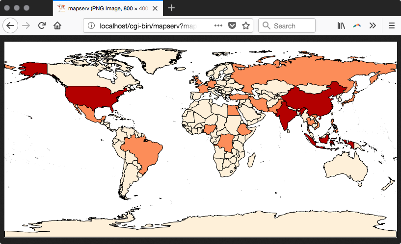
As you can see, there is a small difference between the URLs used in Windows, Linux, and macOS. We will refer to Linux from now on, but you can easily adapt the URLs to Windows or macOS.
<WMT_MS_Capabilities version="1.1.1">
...
<Service>
<Name>OGC:WMS</Name>
<Title>Population per country map</Title>
<Abstract>Map server sample map</Abstract>
<OnlineResource
xmlns:xlink="http://www.w3.org/1999/xlink"
xlink:href="http://localhost/cgi-
bin/mapserv?map=/var/www/data/countries.map&"/>
<ContactInformation> </ContactInformation>
</Service>
<Capability>
<Request>
<GetCapabilities>
...
</GetCapabilities>
<GetMap>
<Format>image/png</Format>
...
<Format>image/tiff</Format>
...
</GetMap>
<GetFeatureInfo>
<Format>text/plain</Format>
...
</GetFeatureInfo>
...
</Request>
...
<Layer>
<Name>population_per_country_map</Name>
<Title>Population per country map</Title>
<Abstract>OWS service about population per country map
in 2005</Abstract>
<SRS>EPSG:4326</SRS>
<SRS>EPSG:3857</SRS>
<LatLonBoundingBox minx="-180" miny="-90" maxx="180"
maxy="90" />
...
</Layer>
</Layer>
</Capability>
</WMT_MS_Capabilities>
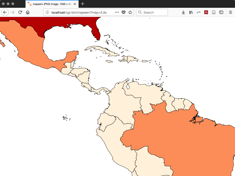
http://localhost/cgi-bin/mapserv?map=/var/www/data/
countries.map&layer=countries&REQUEST=GetFeatureInfo&
SERVICE=WMS&VERSION=1.1.1&LAYERS=countries&
QUERY_LAYERS=countries&SRS=EPSG:4326&BBOX=-122.545074509804,
37.6736653056517,-122.35457254902,37.8428758708189&
X=652&Y=368&WIDTH=1020&HEIGHT=906&INFO_FORMAT=text/html
The output should be as follows:
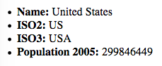
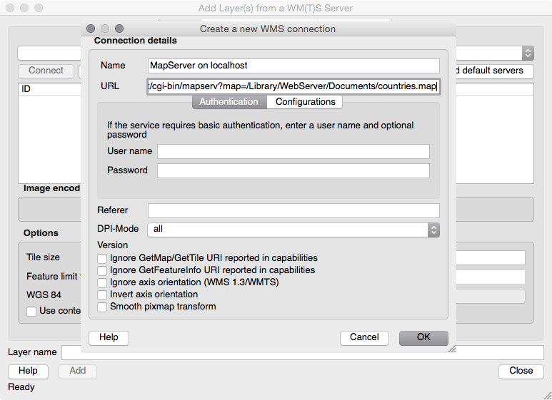
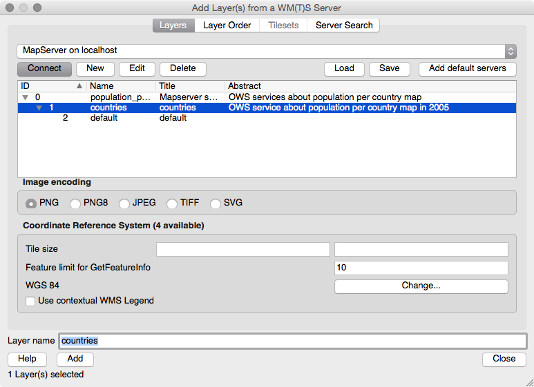
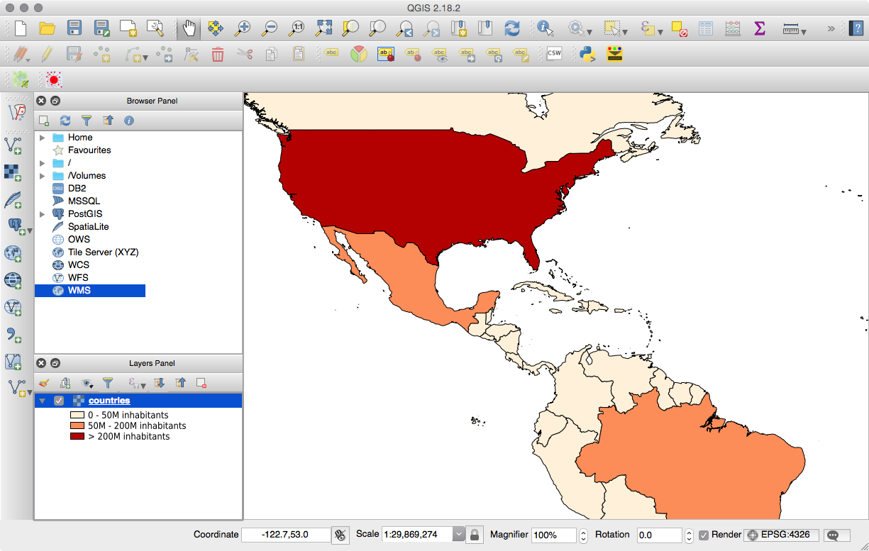
<gml:featureMember>
<ms:countries>
<gml:boundedBy>
<gml:Box srsName="EPSG:4326">
<gml:coordinates>-61.891113,16.989719 -
61.666389,17.724998</gml:coordinates>
</gml:Box>
</gml:boundedBy>
<ms:msGeometry>
<gml:MultiPolygon srsName="EPSG:4326">
<gml:polygonMember>
<gml:Polygon>
<gml:outerBoundaryIs>
<gml:LinearRing>
<gml:coordinates>
-61.686668,17.024441 ...
</gml:coordinates>
</gml:LinearRing>
</gml:outerBoundaryIs>
</gml:Polygon>
</gml:polygonMember>
...
</gml:MultiPolygon>
</ms:msGeometry>
<ms:gid>1</ms:gid>
<ms:fips>AC</ms:fips>
<ms:iso2>AG</ms:iso2>
<ms:iso3>ATG</ms:iso3>
<ms:un>28</ms:un>
<ms:name>Antigua and Barbuda</ms:name>
<ms:area>44</ms:area>
<ms:pop2005>83039</ms:pop2005>
<ms:region>19</ms:region>
<ms:subregion>29</ms:subregion>
<ms:lon>-61.783</ms:lon>
<ms:lat>17.078</ms:lat>
</ms:countries>
</gml:featureMember>
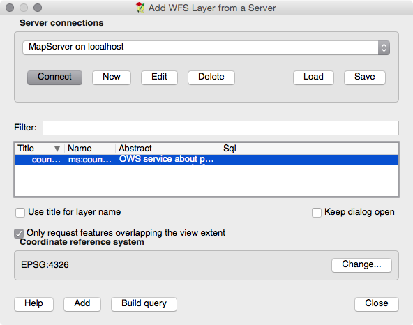
You should now be able to see the vector map in QGIS and inspect the features:
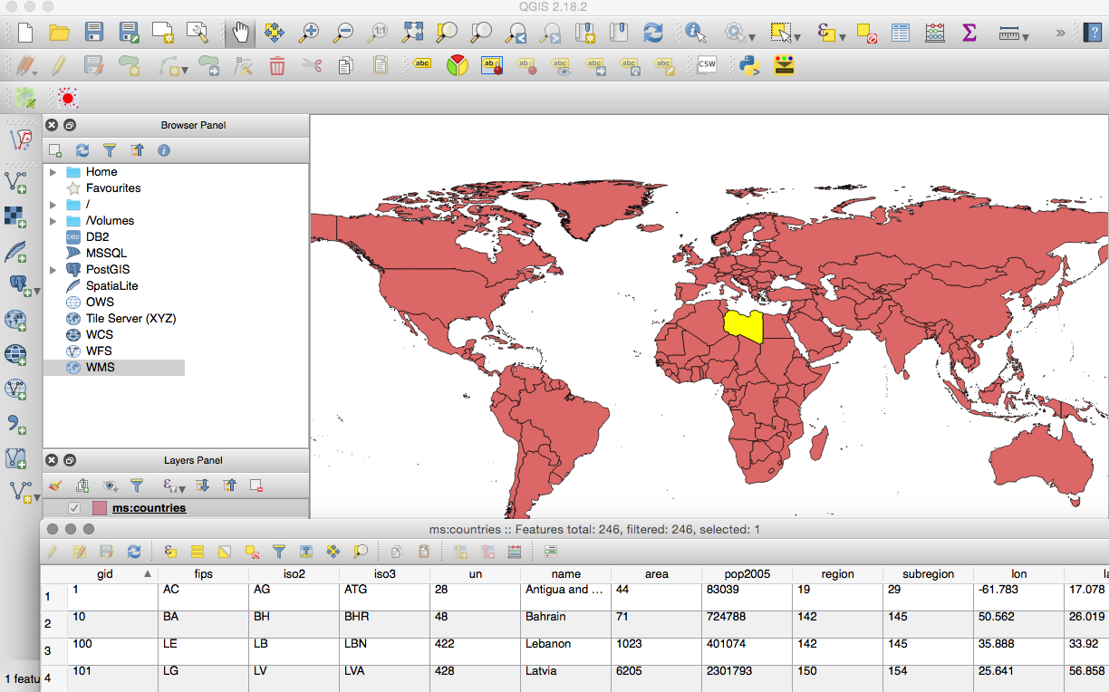
In this recipe, you implemented WMS and WFS services for a PostGIS layer using the MapServer open source web-mapping engine. WMS and WFS are the two core concepts to consider when you want to develop a web GIS that is interoperable across many organizations. Open Geospatial Consortium (OGC) defined these two standards (and many others) to make web-mapping services exposed in an open, standard way. This way these services can be used by different applications; for example, you have seen in this recipe that a GIS Desktop tool such as QGIS can browse and query those services because it understands these OGC standards (you can get exactly the same results with other tools, such as gvSIG, uDig, OpenJUMP, and ArcGIS Desktop, among others). In the same way, Javascript API libraries, most notably OpenLayers and Leaflet (you will be using these in the other recipes in this chapter), can use these services in a standard way to provide web-mapping features to web applications.
WMS is a service that is used to generate the maps to be displayed by clients. Those maps are generated using image formats, such as PNG, JPEG, and many others. Some of the most typical WMS requests are as follows:
WFS provides a convenient, standard way to access the features of a vector layer with a web request. The service response streams to the client the requested features using GML (an XML markup defined by OGC to define geographical features).
Some WFS requests are as follows:
These WMS and WFS requests can be consumed by the client using the HTTP protocol. You have seen how to query and get a response from the client by typing a URL in a browser with several parameters appended to it. As an example, the following WMS GetMap request will return a map image of the layers (using the LAYERS parameter) in a specified format (using the FORMAT parameter), size (using the WIDTH and HEIGHT parameters), extent (using the BBOX parameter), and spatial reference system (using CRS):
http://localhost/cgi-bin/mapserv?map=/var/www/data/countries.map&&SERVICE=WMS&VERSION=1.3.0&REQUEST=GetMap&BBOX=-26,-111,36,-38&CRS=EPSG:4326&WIDTH=806&HEIGHT=688&LAYERS=countries&STYLES=&FORMAT=image/png
In MapServer, you can create WMS and WFS services in the mapfile using its directives. The mapfile is a text file that is composed of several sections and is the heart of MapServer. In the beginning of the mapfile, it is necessary to define general properties for the map, such as its title, extent, spatial reference, output-image formats, and dimensions to be returned to the user.
Then, it is possible to define which OWS (OGC web services such as WMS, WFS, and WCS) requests to expose.
Then there is the main section of the mapfile, where the layers are defined (every layer is defined in the LAYER directive). You have seen how to define a PostGIS layer. It is necessary to define its connection information (database, user, password, and so on), the SQL definition in the database (it is possible to use just a PostGIS table name, but you could eventually use a query to define the set of features and attributes defining the layer), the geometric type, and the projection.
A whole directive (CLASS) is used to define how the layer features will be rendered. You may use different classes, as you did in this recipe, to render features differently, based on an attribute defined with the CLASSITEM setting. In this recipe, you defined three different classes, each representing a population class, using different colors.
In the previous recipe, you created WMS and WFS from a PostGIS layer using MapServer. In this recipe, you will do it using another popular open source web-mapping engine-GeoServer. You will then use the created services as you did with MapServer, testing their exposed requests, first using a browser and then the QGIS desktop tool (you can do this with other software, such as uDig, gvSIG, OpenJUMP GIS, and ArcGIS Desktop).
While MapServer is written in the C language and uses Apache as its web server, GeoServer is written in Java and you therefore need to install the Java Virtual Machine (JVM) in your system; it must be used from a servlet container, such as Jetty and Tomcat. After installing the servlet container, you will be able to deploy the GeoServer application to it. For example, in Tomcat, you can deploy GeoServer by copying the GeoServer WAR (web archive) file to Tomcat's webapps directory. For this recipe, we will suppose that you have a working GeoServer in your system; if this is not the case, follow the detailed GeoServer installation steps for your OS at the GeoServer website (http://docs.geoserver.org/stable/en/user/installation/) and then return to this recipe. Follow these steps:
$ ogr2ogr -f PostgreSQL -a_srs EPSG:4326 -lco GEOMETRY_NAME=the_geom
-nln chp09.counties PG:"dbname='postgis_cookbook' user='me'
password='mypassword'" countyp020.shp
Carry out the following steps:
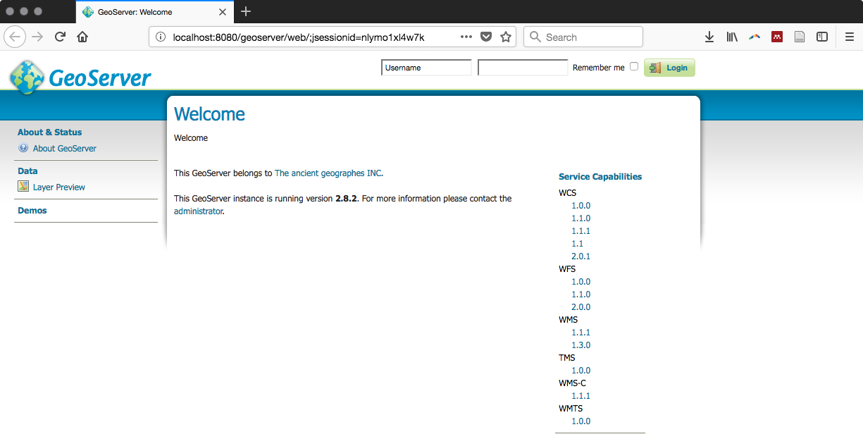
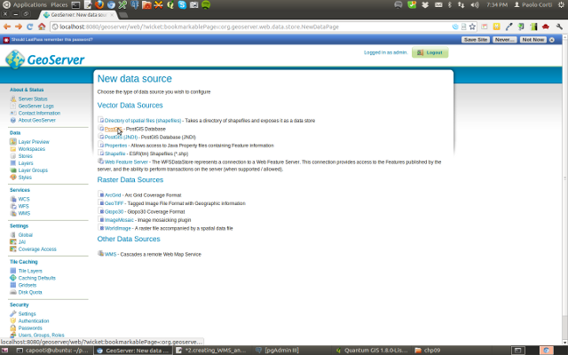
The New Vector Data Source page is shown in the following screenshot:
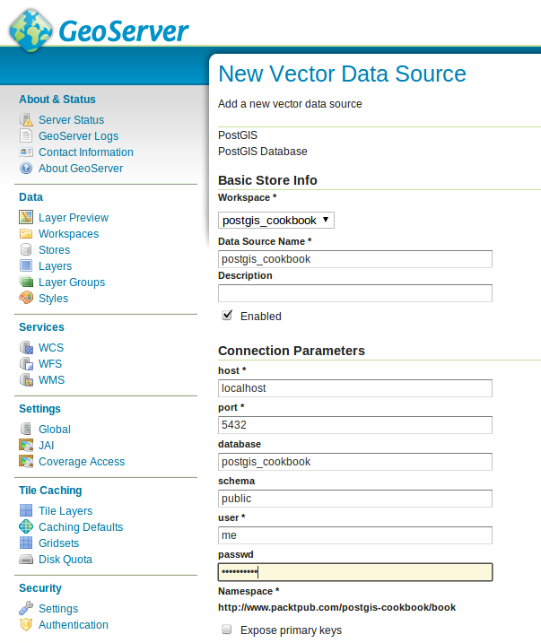
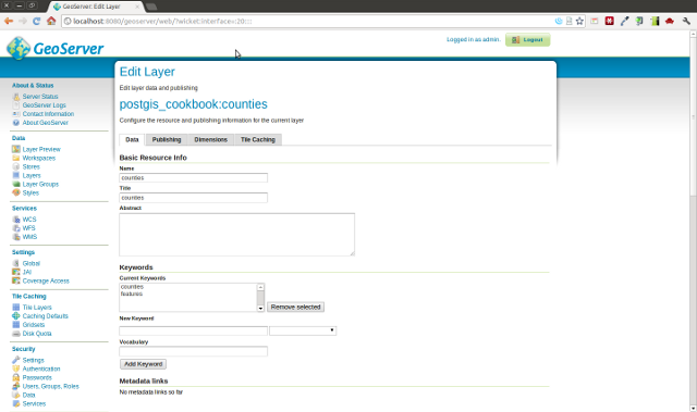
<?xml version="1.0" encoding="UTF-8"?>
<sld:StyledLayerDescriptor xmlns="http://www.opengis.net/sld"
xmlns:sld="http://www.opengis.net/sld"
xmlns:ogc="http://www.opengis.net/ogc"
xmlns:gml="http://www.opengis.net/gml" version="1.0.0">
<sld:NamedLayer>
<sld:Name>county_classification</sld:Name>
<sld:UserStyle>
<sld:Name>county_classification</sld:Name>
<sld:Title>County area classification</sld:Title>
<sld:FeatureTypeStyle>
<sld:Name>name</sld:Name>
<sld:Rule>
<sld:Title>Large counties</sld:Title>
<ogc:Filter>
<ogc:PropertyIsGreaterThanOrEqualTo>
<ogc:PropertyName>square_mil</ogc:PropertyName>
<ogc:Literal>5000</ogc:Literal>
</ogc:PropertyIsGreaterThanOrEqualTo>
</ogc:Filter>
<sld:PolygonSymbolizer>
<sld:Fill>
<sld:CssParameter
name="fill">#FF0000</sld:CssParameter>
</sld:Fill>
<sld:Stroke/>
</sld:PolygonSymbolizer>
</sld:Rule>
<sld:Rule>
<sld:Title>Small counties</sld:Title>
<ogc:Filter>
<ogc:PropertyIsLessThan>
<ogc:PropertyName>square_mil</ogc:PropertyName>
<ogc:Literal>5000</ogc:Literal>
</ogc:PropertyIsLessThan>
</ogc:Filter>
<sld:PolygonSymbolizer>
<sld:Fill>
<sld:CssParameter
name="fill">#0000FF</sld:CssParameter>
</sld:Fill>
<sld:Stroke/>
</sld:PolygonSymbolizer>
</sld:Rule>
</sld:FeatureTypeStyle>
</sld:UserStyle>
</sld:NamedLayer>
</sld:StyledLayerDescriptor>
The following screenshot shows how the new style looks on the New style GeoServer page:
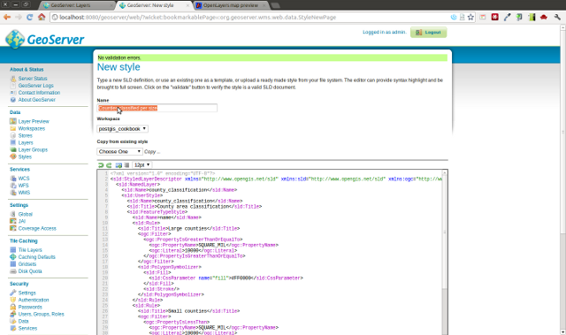
<Layer queryable="1">
<Name>postgis_cookbook:counties</Name>
<Title>counties</Title>
<Abstract/>
<KeywordList>
<Keyword>counties</Keyword>
<Keyword>features</Keyword>
</KeywordList>
<CRS>EPSG:4326</CRS>
<CRS>CRS:84</CRS>
<EX_GeographicBoundingBox>
<westBoundLongitude>-179.133392333984
</westBoundLongitude>
<eastBoundLongitude>-64.566162109375
</eastBoundLongitude>
<southBoundLatitude>17.6746921539307
</southBoundLatitude>
<northBoundLatitude>71.3980484008789
</northBoundLatitude>
</EX_GeographicBoundingBox>
<BoundingBox CRS="CRS:84" minx="-179.133392333984"
miny="17.6746921539307" maxx="-64.566162109375"
maxy="71.3980484008789"/>
<BoundingBox CRS="EPSG:4326" minx="17.6746921539307"
miny="-179.133392333984" maxx="71.3980484008789" maxy="-
64.566162109375"/>
<Style>
<Name>Counties classified per size</Name>
<Title>County area classification</Title>
<Abstract/>
<LegendURL width="20" height="20">
<Format>image/png</Format>
<OnlineResource
xmlns:xlink="http://www.w3.org/1999/xlink"
xlink:type="simple" xlink:href=
"http://localhost:8080/geoserver/
ows?service=WMS&request=GetLegendGraphic&
format=image%2Fpng&width=20&height=20&
layer=counties"/>
</LegendURL>
</Style>
</Layer>
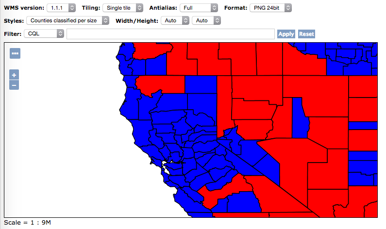
Here is what you get when inspecting the requests with any in-browser developer tool, check the request URL, and verify the parameters sent to geoserver; this is how it looks with Firefox:
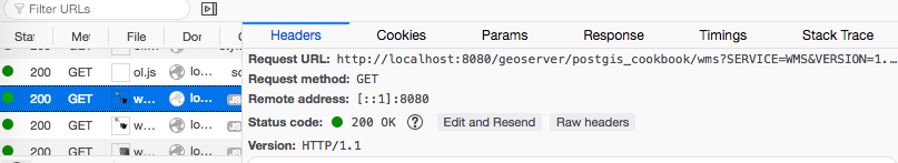
This will be displayed by prompting the previous URL:
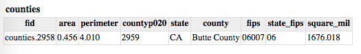

<FeatureType>
<Name>postgis_cookbook:counties</Name>
<Title>counties</Title>
<Abstract/>
<Keywords>counties, features</Keywords>
<SRS>EPSG:4326</SRS>
<LatLongBoundingBox minx="-179.133392333984"
miny="17.6746921539307" maxx="-64.566162109375"
maxy="71.3980484008789"/>
</FeatureType>
<gml:featureMember>
<postgis_cookbook:counties fid="counties.3962">
<postgis_cookbook:the_geom>
<gml:Polygon srsName="http://www.opengis.net/
gml/srs/epsg.xml#4326">
<gml:outerBoundaryIs>
<gml:LinearRing>
<gml:coordinates xmlns:gml=
"http://www.opengis.net/gml"
decimal="." cs="," ts="">
-101.62554932,36.50246048 -
101.0908432,36.50032043 ...
...
...
</gml:coordinates>
</gml:LinearRing>
</gml:outerBoundaryIs>
</gml:Polygon>
</postgis_cookbook:the_geom>
<postgis_cookbook:area>0.240</postgis_cookbook:area>
<postgis_cookbook:perimeter>1.967
</postgis_cookbook:perimeter>
<postgis_cookbook:co2000p020>3963.0
</postgis_cookbook:co2000p020>
<postgis_cookbook:state>TX</postgis_cookbook:state>
<postgis_cookbook:county>Hansford
County</postgis_cookbook:county>
<postgis_cookbook:fips>48195</postgis_cookbook:fips>
<postgis_cookbook:state_fips>48
</postgis_cookbook:state_fips>
<postgis_cookbook:square_mil>919.801
</postgis_cookbook:square_mil>
</postgis_cookbook:counties>
</gml:featureMember>
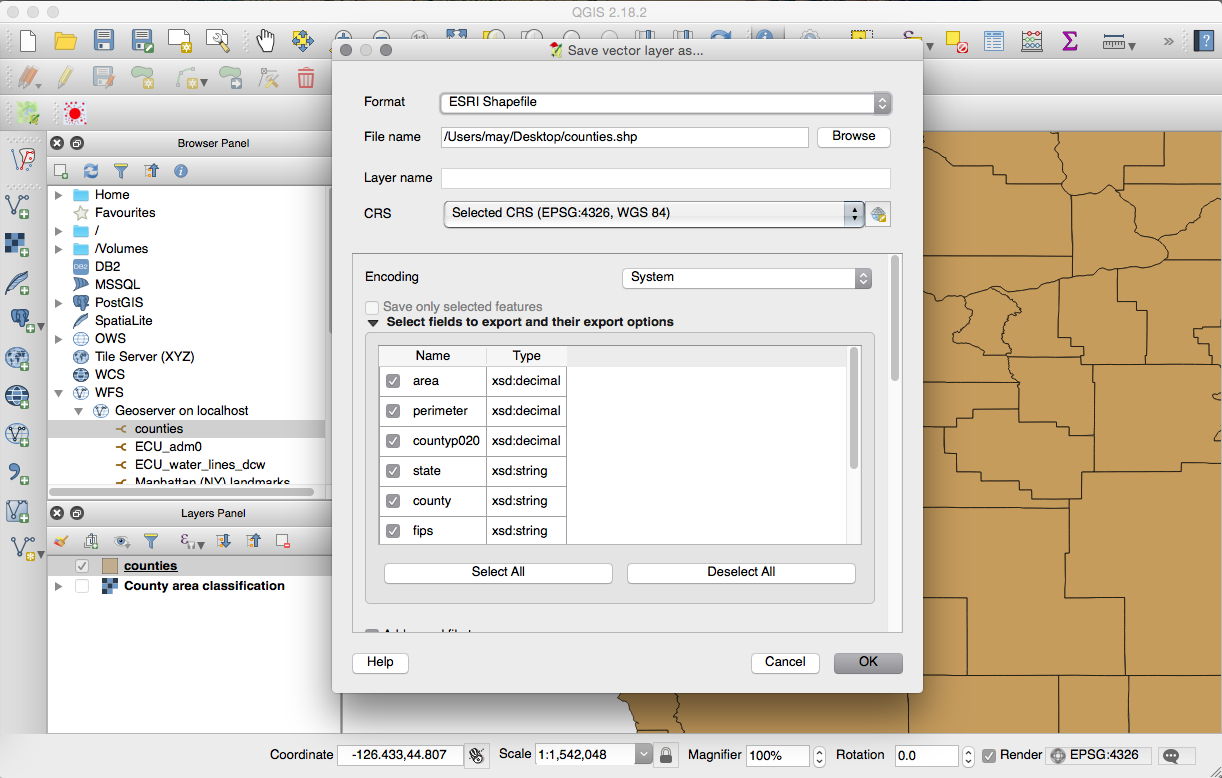
In the previous recipe, you were introduced to the basic concepts of the OGC WMS and WFS standards using MapServer. In this recipe, you have done the same using another popular open source web-mapping engine, GeoServer.
Unlike MapServer, which is written in C and can be used from web servers such as Apache HTTP (HTTPD) or Microsoft Internet Information Server (IIS) as a CGI program, GeoServer is written in Java and needs a servlet container such as Apache Tomcat or Eclipse Jetty to work.
GeoServer not only offers the user a highly scalable and standard web-mapping engine implementation, but does so with a nice user interface, the Web Administration interface. Therefore, it is generally easier for a beginner to create WMS and WFS services compared to MapServer, where it is necessary to master the mapfile syntax.
The GeoServer workflow to create WMS and WFS services for a PostGIS layer is to first create a PostGIS store, where you need to associate the main PostGIS connection parameters (server name, schema, user, and so on). After the store is correctly created, you can publish the layers that are available for that PostGIS store. You have seen in this recipe how easy the whole process is using the GeoServer Web Administration interface.
To define the layer style to render features, GeoServer uses the SLD schema, an OGC standard based on XML. We have written two distinct rules in this recipe to render the counties that have an area greater than 5,000 square miles an area greater than 5,000 square miles in a different way from the others. For the purpose of rendering the counties in a different way, we have used two <ogc:Rule> SLD elements in which you have defined an <ogc:Filter> element. For each of these elements, you have defined the criteria to filter the layer features, using the <ogc:PropertyIsGreaterThanOrEqualTo> and <ogc:PropertyIsLessThan> elements. A very handy way to generate an SLD for a layer is using desktop GIS tools that are able to export an SLD file for a layer (QGIS can do this). After exporting the file, you can upload it to GeoServer by copying the SLD file content to the Add a new style page.
Having created the WMS and WFS services for the counties layer, you have been testing them by generating the requests using the handy Layer Preview GeoServer interface (based on OpenLayers) and then typing the requests directly in a browser. You can modify each service request's parameters from the Layer Preview interface or just by changing them in the URL query string.
Finally, you tested the services using QGIS and have seen how it is possible to export some of the layer's features using the WFS service.
If you want more information about GeoServer, you can check out its excellent documentation at http://docs.geoserver.org/ or get the wonderful GeoServer Beginner's Guide book by Packt Publishing (http://www.packtpub.com/geoserver-share-edit-geospatial-data-beginners-guide/book).
In this recipe, you will implement a WMS Time with MapServer. For time-series data, and whenever you have geographic data that is updated continuously and you need to expose it as a WMS in a Web GIS, WMS Time is the way to go. This is possible by providing the TIME parameter a time value in the WMS requests, typically in the GetMap request.
Here, you will implement a WMS Time service for the hotspots, representing possible fire data acquired by NASA's Earth Observing System Data and Information System (EOSDIS). This excellent system provides data derived from MODIS images from the last 24 hours, 48 hours, and 7 days, which can be downloaded in shapefile, KML, WMS, or text file formats. You will load a bunch of this data to PostGIS, create a WMS Time service with MapServer, and test the WMS GetCapabilities and GetMap requests using a common browser.
$ shp2pgsql -s 4326 -g the_geom -I
MODIS_C6_Global_7d.shp chp09.hotspots > hotspots.sql $ psql -U me -d postgis_cookbook -f hotspots.sql
postgis_cookbook=# SELECT acq_date, count(*) AS hotspots_count
FROM chp09.hotspots GROUP BY acq_date ORDER BY acq_date;
The previous command will produce the following output:
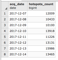
Carry out the following steps:
MAP # Start of mapfile
NAME 'hotspots_time_series'
IMAGETYPE PNG
EXTENT -180 -90 180 90
SIZE 800 400
IMAGECOLOR 255 255 255
# map projection definition
PROJECTION
'init=epsg:4326'
END
# a symbol for hotspots
SYMBOL
NAME "circle"
TYPE ellipse
FILLED true
POINTS
1 1
END
END
# web section: here we define the ows services
WEB
# WMS and WFS server settings
METADATA
'wms_name' 'Hotspots'
'wms_title' 'World hotspots time
series'
'wms_abstract' 'Active fire data detected
by NASA Earth Observing
System Data and Information
System (EOSDIS)'
'wms_onlineresource' 'http://localhost/cgi-bin/
mapserv?map=/var/www/data/
hotspots.map&'
'wms_srs' 'EPSG:4326 EPSG:3857'
'wms_enable_request' '*'
'wms_feature_info_mime_type' 'text/html'
END
END
# Start of layers definition
LAYER # Hotspots point layer begins here
NAME hotspots
CONNECTIONTYPE POSTGIS
CONNECTION 'host=localhost dbname=postgis_cookbook
user=me
password=mypassword port=5432'
DATA 'the_geom from chp09.hotspots'
TEMPLATE 'template.html'
METADATA
'wms_title' 'World hotspots time
series'
'gml_include_items' 'all'
END
STATUS ON
TYPE POINT
CLASS
SYMBOL 'circle'
SIZE 4
COLOR 255 0 0
END # end of class
END # hotspots layer ends here
END # End of mapfile
In the following steps, we will be referring to Linux. If you are using Windows, you just need to replace http://localhost/cgi-bin/mapserv?map=/var/www/data/hotspots.map with http://localhost/cgi-bin/mapserv.exe?map=C:\ms4w\Apache\htdoc\shotspots.map; or if using macOS, replace it with http://localhost/cgi-bin/mapserv?map=/Library/WebServer/Documents/hotsposts.map in every request:
The map displayed on your browser will look as follows:
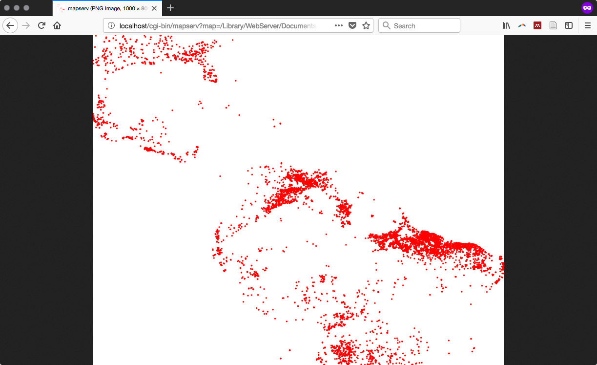
METADATA
'wms_title' 'World hotspots time
series'
'gml_include_items' 'all'
'wms_timeextent' '2000-01-01/2020-12-31' # time extent
for which the service will give a response
'wms_timeitem' 'acq_date' # layer field to use to filter
on the TIME parameter
'wms_timedefault' '2013-05-30' # default parameter if not
added to the request
END
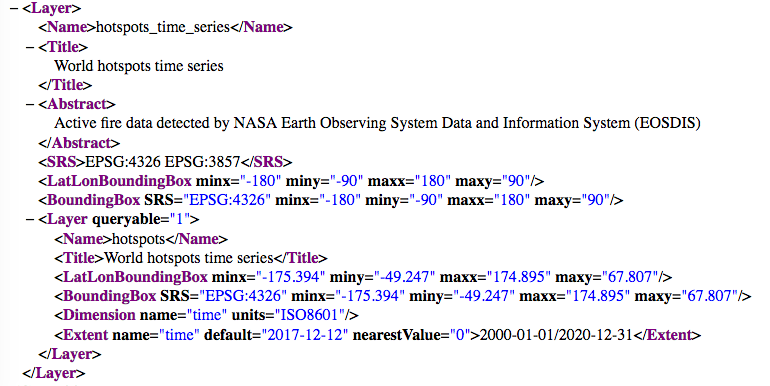
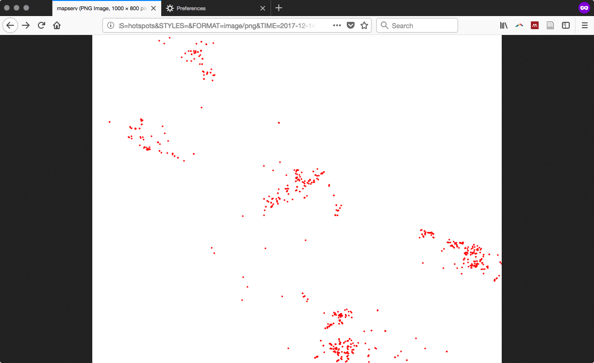
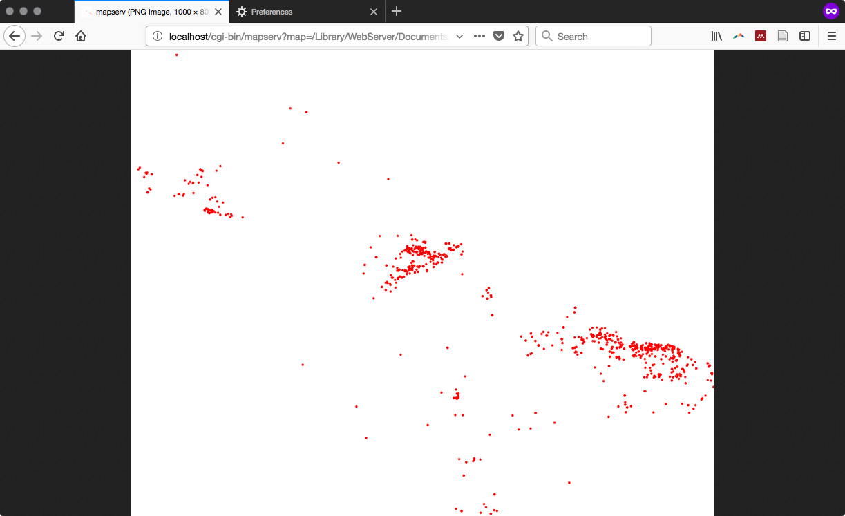
In this recipe, you have seen how to create a WMS Time service using the MapServer open source web-mapping engine. A WMS Time service is useful for whenever you have temporal series and geographic data varying in the time. WMS Time lets the user filter the requested data by providing a TIME parameter with a time value in the WMS requests.
For this purpose, you first created a plain WMS; if you are new to the WMS standard, mapfile, and MapServer, you can check out the first recipe in this chapter. You have imported in PostGIS a points shapefile with one week's worth of hotspots derived from the MODIS satellite and created a simple WMS for this layer.
After verifying that this WMS works well by testing the WMS GetCapabilities and GetMap requests, you have time enabled the WMS by adding three parameters in the LAYER METADATA mapfile section: wms_timeextent, wms_timeitem, and wms_timedefault.
The wms_timeextent parameter is the duration of time in which the service will give a response. It defines the PostGIS table field to be used to filter the TIME parameter (the acq_date field in this case). The wms_timedefault parameter specifies a default time value to be used when the request to the WMS service does not provide the TIME parameter.
At this point, the WMS is time enabled; this means that the WMS GetCapabilities request now includes the time-dimension definition for the PostGIS hotspots layer and, more importantly, the GetMap WMS request lets the user add the TIME parameter to query the layer for a specific date.
In this recipe, you will use the MapServer and Geoserver WMS you created in the first two recipes of this chapter using the OpenLayers open source JavaScript API.
This excellent library helps developers quickly assemble web pages using mapping viewers and features. In this recipe, you will create an HTML page, add an OpenLayers map in it and a bunch of controls in that map for navigation, switch the layers, and identify features of the layers. We will also look at two WMS layers pointing to the PostGIS tables, implemented with MapServer and GeoServer.
MapServer uses PROJ.4 (https://trac.osgeo.org/proj/) for projection management. This library does not exist by default with the Spherical Mercator projection (EPSG:900913) defined. Such a projection is commonly used by commercial map API providers, such as GoogleMaps, Yahoo! Maps, and Microsoft Bing, and can provide excellent base layers for your maps.
For this recipe, we need to have under consideration the following:
Carry out the following steps:
<!doctype html>
<html>
<head>
<title>OpenLayers Example</title>
<script src="http://openlayers.org/api/OpenLayers.js">
</script>
</head>
<body>
</body>
</html>
<div style="width:900px; height:500px" id="map"></div>
<script defer="defer" type="text/javascript">
// instantiate the map object
var map = new OpenLayers.Map("map", {
controls: [],
projection: new OpenLayers.Projection("EPSG:3857")
});
</script>
// add some controls on the map
map.addControl(new OpenLayers.Control.Navigation());
map.addControl(new OpenLayers.Control.PanZoomBar()),
map.addControl(new OpenLayers.Control.LayerSwitcher(
{"div":OpenLayers.Util.getElement("layerswitcher")}));
map.addControl(new OpenLayers.Control.MousePosition());
// set the OSM layer
var osm_layer = new OpenLayers.Layer.OSM();
// set the WMS
var geoserver_url = "http://localhost:8080/geoserver/wms";
var mapserver_url = http://localhost/cgi-
bin/mapserv?map=/var/www/data/countries.map&
// set the WMS
var geoserver_url = "http://localhost:8080/geoserver/wms";
var mapserver_url = http://localhost/cgi-
bin/mapserv.exe?map=C:\\ms4w\\Apache\\
htdocs\\countries.map&
// set the WMS
var geoserver_url = "http://localhost:8080/geoserver/wms";
var mapserver_url = http://localhost/cgi-
bin/mapserv? map=/Library/WebServer/
Documents/countries.map&
// set the GeoServer WMS
var geoserver_wms = new OpenLayers.Layer.WMS( "GeoServer WMS",
geoserver_url,
{
layers: "postgis_cookbook:counties",
transparent: "true",
format: "image/png",
},
{
isBaseLayer: false,
opacity: 0.4
} );
// set the MapServer WMS
var mapserver_wms = new OpenLayers.Layer.WMS( "MapServer WMS",
mapserver_url,
{
layers: "countries",
transparent: "true",
format: "image/png",
},
{
isBaseLayer: false
} );
// add all of the layers to the map
map.addLayers([mapserver_wms, geoserver_wms, osm_layer]);
map.zoomToMaxExtent();
Proxy...
// add the WMSGetFeatureInfo control
OpenLayers.ProxyHost = "/cgi-bin/proxy.cgi?url=";
var info = new OpenLayers.Control.WMSGetFeatureInfo({
url: geoserver_url,
title: 'Identify',
queryVisible: true,
eventListeners: {
getfeatureinfo: function(event) {
map.addPopup(new OpenLayers.Popup.FramedCloud(
"WMSIdentify",
map.getLonLatFromPixel(event.xy),
null,
event.text,
null,
true
));
}
}
});
map.addControl(info);
info.activate();
// center map
var cpoint = new OpenLayers.LonLat(-11000000, 4800000);
map.setCenter(cpoint, 3);
Your HTML file should now look like the openlayers.html file contained in data/chp09. You can finally deploy this file to your web server (Apache HTTPD or IIS). If you are using Apache HTTPD in Linux, you could copy the file to the data directory under /var/www, and if you are using Windows, you could copy it to the data directory under C:\ms4w\Apache\htdocs (create the data directory if it does not already exist). Then, access it using the URL http://localhost/data/openlayers.html.
Now, access the openlayers web page using your favorite browser. Start browsing the map: zoom, pan, try to switch the base and overlays layers on and off using the layer switcher control, and try to click on a point to identify one feature from the counties PostGIS layer. A map is shown in the following screenshot:
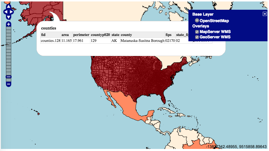
You have seen how to create a web map viewer with the OpenLayers JavaScript library. This library lets the developer define the various map components, using JavaScript in an HTML page. The core object is a map that is composed of controls and layers.
OpenLayers comes with a great number of controls (http://dev.openlayers.org/docs/files/OpenLayers/Control-js.html), and it is even possible to create custom ones.
Another great OpenLayers feature is the ability to add a good number of geographic data sources as layers in the map (you added just a couple of its types to the map, such as OpenStreetMap and WMS) and you could add sources, such as WFS, GML, KML, GeoRSS, OSM data, ArcGIS Rest, TMS, WMTS, and WorldWind, just to name a few.
In the previous recipe, you have seen how to create a webGIS using the OpenLayers JavaScript API and then added the WMS PostGIS layers served from MapServer and GeoServer .
A lighter alternative to the widespread OpenLayers JavaScript API was created, named Leaflet. In this recipe, you will see how to use this JavaScript API to create a webGIS, add a WMS layer from PostGIS to this map, and implement an identify tool, sending a GetFeatureInfo request to the MapServer WMS. However, unlike OpenLayers, Leaflet does not come with a WMSGetFeatureInfo control, so we will see in this recipe how to create this functionality.
Carry out the following steps:
<html>
<head>
<title>Leaflet Example</title>
<link rel="stylesheet"
href= "https://unpkg.com/leaflet@1.2.0/dist/leaflet.css" />
<script src= "https://unpkg.com/leaflet@1.2.0/dist/leaflet.js">
</script>
<script src="http://ajax.googleapis.com/ajax/
libs/jquery/1.9.1/jquery.min.js">
</script>
</head>
<body>
</body>
</html>
<div id="map" style="width:800px; height:500px"></div>
<script defer="defer" type="text/javascript">
// osm layer
var osm = L.tileLayer('http://{s}.tile.osm.org
/{z}/{x}/{y}.png', {
maxZoom: 18,
attribution: "Data by OpenStreetMap"
});
</script>
// mapserver layer
var ms_url = "http://localhost/cgi-bin/mapserv?
map=/var/www/data/countries.map&";
var countries = L.tileLayer.wms(ms_url, {
layers: 'countries',
format: 'image/png',
transparent: true,
opacity: 0.7
});
// mapserver layer
var ms_url = "http://localhost
/cgi-bin/mapserv.exe?map=C:%5Cms4w%5CApache%5
Chtdocs%5Ccountries.map&";
var countries = L.tileLayer.wms(ms_url, {
layers: 'countries',
format: 'image/png',
transparent: true,
opacity: 0.7
});
// mapserver layer
var ms_url = "http://localhost/cgi-bin/mapserv?
map=/Library/WebServer/Documents/countries.map&";
var countries = L.tileLayer.wms(ms_url, {
layers: 'countries',
format: 'image/png',
transparent: true,
opacity: 0.7
});
// map creation
var map = new L.Map('map', {
center: new L.LatLng(15, 0),
zoom: 2,
layers: [osm, countries],
zoomControl: true
});
// getfeatureinfo event
map.addEventListener('click', Identify);
function Identify(e) {
// set parameters needed for GetFeatureInfo WMS request
var BBOX = map.getBounds().toBBoxString();
var WIDTH = map.getSize().x;
var HEIGHT = map.getSize().y;
var X = map.layerPointToContainerPoint(e.layerPoint).x;
var Y = map.layerPointToContainerPoint(e.layerPoint).y;
// compose the URL for the request
var URL = ms_url + 'SERVICE=WMS&VERSION=1.1.1&
REQUEST=GetFeatureInfo&LAYERS=countries&
QUERY_LAYERS=countries&BBOX='+BBOX+'&FEATURE_COUNT=1&
HEIGHT='+HEIGHT+'&WIDTH='+WIDTH+'&
INFO_FORMAT=text%2Fhtml&SRS=EPSG%3A4326&X='+X+'&Y='+Y;
//send the asynchronous HTTP request using
jQuery $.ajax
$.ajax({
url: URL,
dataType: "html",
type: "GET",
success: function(data) {
var popup = new L.Popup({
maxWidth: 300
});
popup.setContent(data);
popup.setLatLng(e.latlng);
map.openPopup(popup);
}
});
}
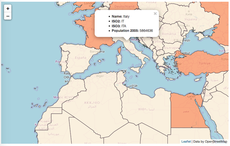
In this recipe, you have seen how to use the Leaflet JavaScript API library to add a map in an HTML page. First, you created one layer from an external server to use as the base map. Then, you created another layer using the MapServer WMS you implemented in a previous recipe to expose a PostGIS layer to the web. Then, you created a new map object and added it to these two layers. Finally, using jQuery, you implemented an AJAX call to the GetFeatureInfo WMS request and displayed the results in a Leaflet Popup object.
Leaflet is a very nice and compact alternative to the OpenLayers library and gives very good results when your webGIS service needs to be used from mobile devices, such as tablets and smart phones. Additionally, it has a plethora of plugins and can be easily integrated with JavaScript libraries, such as Raphael and JS3D.
In this recipe, you will create the Transactional Web Feature Service (WFS-T) from a PostGIS layer with the GeoServer open source web-mapping engine and then an OpenLayers basic application that will be able to use this service.
This way, the user of the application will be able to manage transactions on the remote PostGIS layer. WFS-T allows for the creation, deletion, and updating of features. In this recipe, you will allow the user to only to add features, but this recipe should put you on your way to creating more composite use cases.
If you are new to GeoServer and OpenLayers, you should first read the Creating WMS and WFS services with GeoServer and Consuming WMS services with OpenLayers recipes and then return to this one.
CREATE TABLE chp09.sites
(
gid serial NOT NULL,
the_geom geometry(Point,4326),
CONSTRAINT sites_pkey PRIMARY KEY (gid )
);
CREATE INDEX sites_the_geom_gist ON chp09.sites
USING gist (the_geom );
Carry out the following steps:
<html>
<head>
<title>Consuming a WFS-T with OpenLayers</title>
<script
src="http://openlayers.org/api/OpenLayers.js">
</script>
</head>
<body>
</body>
</html>
<div style="width:700px; height:400px" id="map"></div>
<script type="text/javascript">
// set the proxy
OpenLayers.ProxyHost = "/cgi-bin/proxy.cgi?url=";
// create the map
var map = new OpenLayers.Map('map');
</script>
// create an OSM base layer
var osm = new OpenLayers.Layer.OSM();
// create the wfs layer
var saveStrategy = new OpenLayers.Strategy.Save();
var wfs = new OpenLayers.Layer.Vector("Sites",
{
strategies: [new OpenLayers.Strategy.BBOX(), saveStrategy],
projection: new OpenLayers.Projection("EPSG:4326"),
styleMap: new OpenLayers.StyleMap({
pointRadius: 7,
fillColor: "#FF0000"
}),
protocol: new OpenLayers.Protocol.WFS({
version: "1.1.0",
srsName: "EPSG:4326",
url: "http://localhost:8080/geoserver/wfs",
featurePrefix: 'postgis_cookbook',
featureType: "sites",
featureNS: "https://www.packtpub.com/application-development/
postgis-cookbook-second-edition",
geometryName: "the_geom"
})
});
// add layers to map and center it
map.addLayers([osm, wfs]);
var fromProjection = new OpenLayers.Projection("EPSG:4326");
var toProjection = new OpenLayers.Projection("EPSG:900913");
var cpoint = new OpenLayers.LonLat(12.5, 41.85).transform(
fromProjection, toProjection);
map.setCenter(cpoint, 10);
// create a panel for tools
var panel = new OpenLayers.Control.Panel({
displayClass: "olControlEditingToolbar"
});
// create a draw point tool
var draw = new OpenLayers.Control.DrawFeature(
wfs, OpenLayers.Handler.Point,
{
handlerOptions: {freehand: false, multi: false},
displayClass: "olControlDrawFeaturePoint"
}
);
// create a save tool
var save = new OpenLayers.Control.Button({
title: "Save Features",
trigger: function() {
saveStrategy.save();
},
displayClass: "olControlSaveFeatures"
});
// add tools to panel and add it to map
panel.addControls([
new OpenLayers.Control.Navigation(),
save, draw
]);
map.addControl(panel);
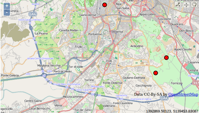
In this recipe, you first created a point PostGIS table and then published it as WFS-T, using GeoServer. You then created a basic OpenLayers application, using the WFS-T layer, allowing the user to add features to the underlying PostGIS layer.
In OpenLayers, the core object needed to implement such a service is the vector layer by defining a WFS protocol. When defining the WFS protocol, you have to provide the WFS version that is using the spatial reference system of the dataset, the URI of the service, the name of the layer (for GeoServer, the name is a combination of the layer workspace, FeaturePrefix, and the layer name, FeatureType), and the name of the geometry field that will be modified. You also can pass to the Vector layer constructor a StyleMap value to define the layer's rendering behavior.
You then tested the application by adding some points to the OpenLayers map and checked that those points were effectively stored in PostGIS. When adding the points using the WFS-T layer, with the help of tools such as Firefox Firebug or Chrome (Chromium) Developer Tools, you could dig in detail into the requests that you are making to the WFS-T and its responses.
For example, when adding a point, you will see that an Insert request is sent to WFS-T. The following XML is sent to the service (note how the point geometry is inserted in the body of the <wfs:Insert> element):
<wfs:Transaction xmlns:wfs="http://www.opengis.net/wfs"
service="WFS" version="1.1.0"
xsi:schemaLocation="http://www.opengis.net/wfs
http://schemas.opengis.net/wfs/1.1.0/wfs.xsd"
xmlns:xsi="http://www.w3.org/2001/XMLSchema-instance"> <wfs:Insert> <feature:sites xmlns:feature="http://www.packtpub.com/
postgis-cookbook/book"> <feature:the_geom> <gml:Point xmlns:gml="http://www.opengis.net/gml"
srsName="EPSG:4326">
<gml:pos>12.450561523436999 41.94302128455888</gml:pos>
</gml:Point> </feature:the_geom> </feature:sites> </wfs:Insert> </wfs:Transaction>
The <wfs:TransactionResponse> response, as shown in the following code, will be sent from WFS-T if the process has transpired smoothly and the features have been stored (note that the <wfs:totalInserted> element value in this case is set to 1, as only one feature was stored):
<?xml version="1.0" encoding="UTF-8"?> <wfs:TransactionResponse version="1.1.0" ...[CLIP]... > <wfs:TransactionSummary>
<wfs:totalInserted>1</wfs:totalInserted>
<wfs:totalUpdated>0</wfs:totalUpdated>
<wfs:totalDeleted>0</wfs:totalDeleted>
</wfs:TransactionSummary> <wfs:TransactionResults/> <wfs:InsertResults> <wfs:Feature> <ogc:FeatureId fid="sites.17"/> </wfs:Feature> </wfs:InsertResults> </wfs:TransactionResponse>
In this recipe and the next, you will use the Django web framework to create a web application to manage wildlife sightings using a PostGIS data store. In this recipe, you will build the back office of the web application, based on the Django admin site.
Upon accessing the back office, an administrative user will be able to, after authentication, manage (insert, update, and delete) the main entities (animals and sightings) of the database. In the next part of the recipe, you will build a front office that displays the sightings on a map based on the Leaflet JavaScript library.
$ cd ~/virtualenvs/
$ virtualenv --no-site-packages chp09-env
$ source chp09-env/bin/activate
cd c:\virtualenvs
C:\Python27\Scripts\virtualenv.exe
-no-site-packages chp09-env
chp09-env\Scripts\activate
(chp09-env)$ pip install django==1.10
(chp09-env)$ pip install psycopg2==2.7
(chp09-env)$ pip install Pillow
(chp09-env) C:\virtualenvs> pip install django==1.10
(chp09-env) C:\virtualenvs> pip install psycopg2=2.7
(chp09-env) C:\virtualenvs> easy_install Pillow
Carry out the following steps:
(chp09-env)$ cd ~/postgis_cookbook/working/chp09
(chp09-env)$ django-admin.py startproject wildlife
(chp09-env)$ cd wildlife/
(chp09-env)$ django-admin.py startapp sightings
Now you should have the following directory structure:
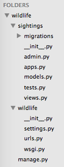
DATABASES = {
'default': {
'ENGINE': 'django.contrib.gis.db.backends.postgis',
'NAME': 'postgis_cookbook',
'USER': 'me',
'PASSWORD': 'mypassword',
'HOST': 'localhost',
'PORT': '',
}
}
import os
PROJECT_PATH = os.path.abspath(os.path.dirname(__file__))
MEDIA_ROOT = os.path.join(PROJECT_PATH, "media")
MEDIA_URL = '/media/'
INSTALLED_APPS = (
'django.contrib.admin',
'django.contrib.auth',
'django.contrib.contenttypes',
'django.contrib.sessions',
'django.contrib.messages',
'django.contrib.staticfiles',
'django.contrib.gis',
'sightings',
)
(chp09-env)$ python manage.py makemigrations
(chp09-env)$ python manage.py migrate
from django.db import models
from django.contrib.gis.db import models as gismodels
class Country(gismodels.Model):
"""
Model to represent countries.
"""
isocode = gismodels.CharField(max_length=2)
name = gismodels.CharField(max_length=255)
geometry = gismodels.MultiPolygonField(srid=4326)
objects = gismodels.GeoManager()
def __unicode__(self):
return '%s' % (self.name)
class Animal(models.Model):
"""
Model to represent animals.
"""
name = models.CharField(max_length=255)
image = models.ImageField(upload_to='animals.images')
def __unicode__(self):
return '%s' % (self.name)
def image_url(self):
return u'<img src="%s" alt="%s" width="80"></img>' %
(self.image.url, self.name)
image_url.allow_tags = True
class Meta:
ordering = ['name']
class Sighting(gismodels.Model):
"""
Model to represent sightings.
"""
RATE_CHOICES = (
(1, '*'),
(2, '**'),
(3, '***'),
)
date = gismodels.DateTimeField()
description = gismodels.TextField()
rate = gismodels.IntegerField(choices=RATE_CHOICES)
animal = gismodels.ForeignKey(Animal)
geometry = gismodels.PointField(srid=4326)
objects = gismodels.GeoManager()
def __unicode__(self):
return '%s' % (self.date)
class Meta:
ordering = ['date']
from django.contrib import admin
from django.contrib.gis.admin import GeoModelAdmin
from models import Country, Animal, Sighting
class SightingAdmin(GeoModelAdmin):
"""
Web admin behavior for the Sighting model.
"""
model = Sighting
list_display = ['date', 'animal', 'rate']
list_filter = ['date', 'animal', 'rate']
date_hierarchy = 'date'
class AnimalAdmin(admin.ModelAdmin):
"""
Web admin behavior for the Animal model.
"""
model = Animal
list_display = ['name', 'image_url',]
class CountryAdmin(GeoModelAdmin):
"""
Web admin behavior for the Country model.
"""
model = Country
list_display = ['isocode', 'name']
ordering = ('name',)
class Meta:
verbose_name_plural = 'countries'
admin.site.register(Animal, AnimalAdmin)
admin.site.register(Sighting, SightingAdmin)
admin.site.register(Country, CountryAdmin)
(chp09-env)$ python manage.py makemigrations
(chp09-env)$ python manage.py migrate
The output should be as follows:
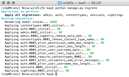
from django.conf.urls import url
from django.contrib import admin
import settings
from django.conf.urls.static import static
admin.autodiscover()
urlpatterns = [
url(r'^admin/', admin.site.urls),
] + static(settings.MEDIA_URL, document_root=settings.MEDIA_ROOT)
In the urls.py file, you basically defined the location of the back office (which was built using the Django admin application) and the media (images) files' location uploaded by the Django administrator when adding new animal entities in the database. Now run the Django development server, using the following runserver management command:
(chp09-env)$ python manage.py runserver
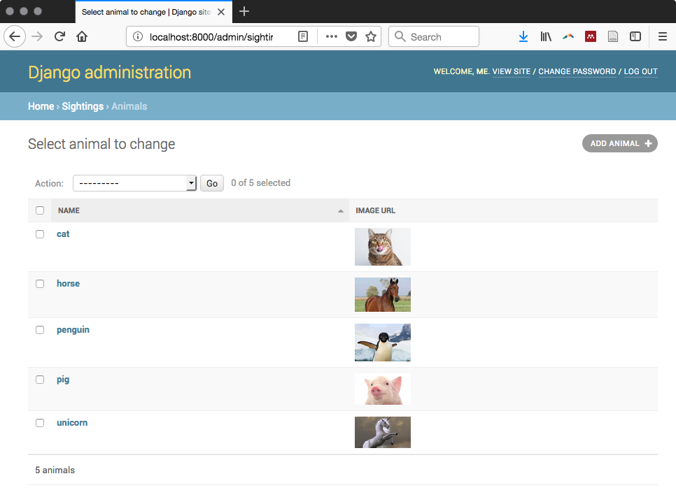
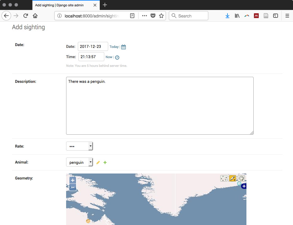
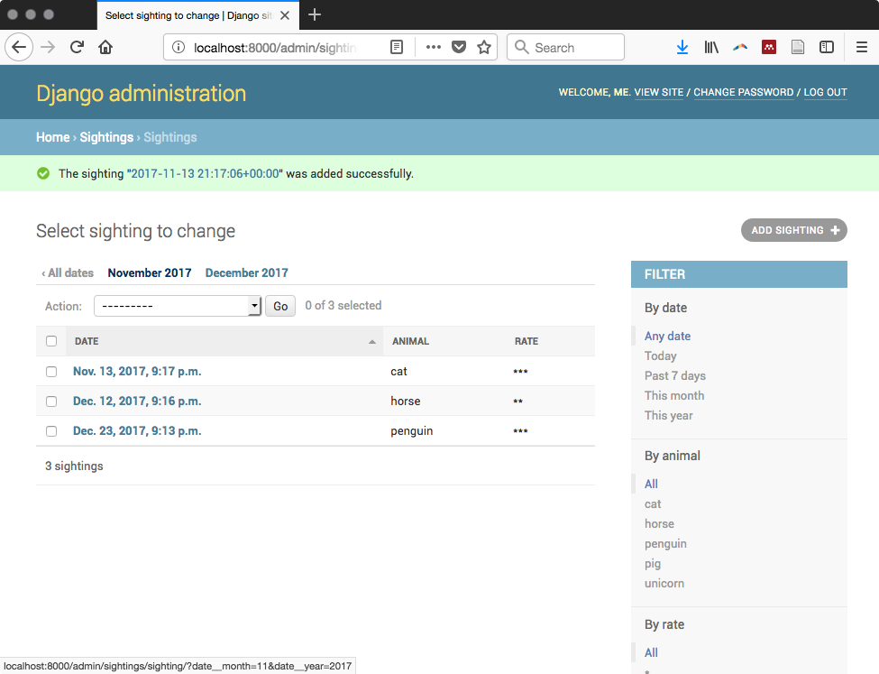
$ ogrinfo TM_WORLD_BORDERS-0.3.shp TM_WORLD_BORDERS-0.3 -al -so
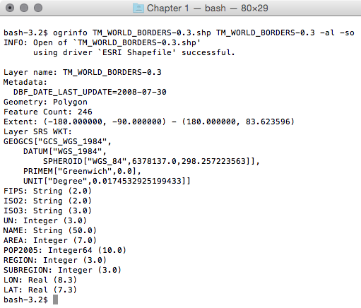
"""
Script to load the data for the country model from a shapefile.
"""
from django.contrib.gis.utils import LayerMapping
from models import Country
country_mapping = {
'isocode' : 'ISO2',
'name' : 'NAME',
'geometry' : 'MULTIPOLYGON',
}
country_shp = 'TM_WORLD_BORDERS-0.3.shp'
country_lm = LayerMapping(Country, country_shp, country_mapping,
transform=False, encoding='iso-8859-1')
country_lm.save(verbose=True, progress=True)
(chp09-env)$ python manage.py shell
>>> from sightings import load_countries
Saved: Antigua and Barbuda
Saved: Algeria Saved: Azerbaijan
...
Saved: Taiwan
Now, you should see the countries in the administrative interface at http://localhost:8000/admin/sightings/country/, while running the Django server with:
(chp09-env)$ python manage.py runserver
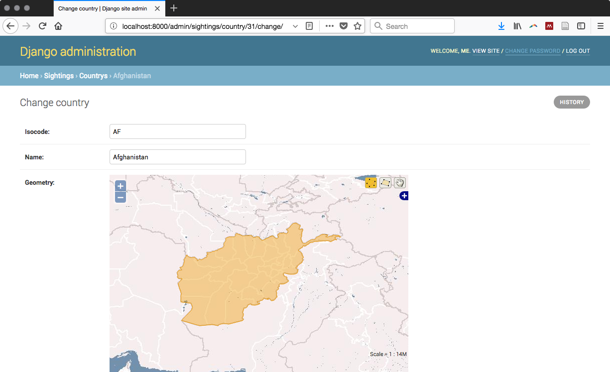
In this recipe, you have seen how quick and efficient it is to assemble a back office application using Django, one of the most popular Python web frameworks; this is thanks to its object-relational mapper, which automatically created the database tables needed by your application and an automatic API to manage (insert, update, and delete) and query the entities without using SQL.
Thanks to the GeoDjango library, two of the application models, County and Sighting, have been geo-enabled with their introduction in the database tables of geometric PostGIS fields.
You have customized the powerful automatic administrative interface to quickly assemble the back-office pages of your application. Using the Django URL Dispatcher, you have defined the URL routes for your application in a concise manner.
As you may have noticed, what is extremely nice about the Django abstraction is the automatic implementation of the data-access layer API using the models. You can now add, update, delete, and query records using Python code, without having any knowledge of SQL. Try this yourself, using the Django Python shell; you will select an animal from the database, add a new sighting for that animal, and then finally delete the sighting. You can investigate the SQL generated by Django, behind the scenes, any time, using the django.db.connection class with the following command:
(chp09-env-bis)$ python manage.py shell
>>> from django.db import connection
>>> from datetime import datetime
>>> from sightings.models import Sighting, Animal
>>> an_animal = Animal.objects.all()[0]
>>> an_animal
<Animal: Lion>
>>> print connection.queries[-1]['sql']
SELECT "sightings_animal"."id", "sightings_animal"."name", "sightings_animal"."image" FROM "sightings_animal" ORDER BY "sightings_animal"."name" ASC LIMIT 1'
my_sight = Sighting(date=datetime.now(), description='What a lion I have seen!', rate=1, animal=an_animal, geometry='POINT(10 10)')
>>> my_sight.save()
print connection.queries[-1]['sql']
INSERT INTO "sightings_sighting" ("date", "description", "rate", "animal_id", "geometry") VALUES ('2013-06-12 14:37:36.544268-05:00', 'What a lion I have seen!', 1, 2, ST_GeomFromEWKB('\x0101000020e610000000000000000024400000000000002440'::bytea)) RETURNING "sightings_sighting"."id"
>>> my_sight.delete()
>>> print connection.queries[-1]['sql']
DELETE FROM "sightings_sighting" WHERE "id" IN (5)
Do you like Django as much as we do? In the next recipe, you will create the frontend of the application. The user will be able to browse the sightings in a map, implemented with the Leaflet JavaScript library. So keep reading!
In this recipe, you will create the front office for the web application you created using Django in the previous recipe.
Using HTML and the Django template language, you will create a web page displaying a map, implemented with Leaflet, and a list for the user containing all of the sightings available in the system. The user will be able to navigate the map and identify the sightings to get more information.
$ cd ~/virtualenvs/ $ source chp09-env/bin/activate
cd c:\virtualenvs > chp09-env\Scripts\activate
(chp09-env)$ pip install simplejson
(chp09-env)$ pip install vectorformats
(chp09-env) C:\virtualenvs> pip install simplejson
(chp09-env) C:\virtualenvs> pip install vectorformats
You will now create the front page of your web application, as follows:
from django.conf.urls import patterns, include, url
from django.conf import settings
from sightings.views import get_geojson, home
from django.contrib import admin
admin.autodiscover()
urlpatterns = [
url(r'^admin/', admin.site.urls),
url(r'^geojson/', get_geojson),
url(r'^$', home),
] + static(settings.MEDIA_URL, document_root=settings.MEDIA_ROOT)
# media files
from django.shortcuts import render
from django.http import HttpResponse
from vectorformats.Formats import Django, GeoJSON
from models import Sighting
def home(request):
"""
Display the home page with the list and a map of the sightings.
"""
sightings = Sighting.objects.all()
return render("sightings/home.html", {'sightings' : sightings})
def get_geojson(request):
"""
Get geojson (needed by the map) for all of the sightings.
"""
sightings = Sighting.objects.all()
djf = Django.Django(geodjango='geometry',
properties=['animal_name', 'animal_image_url', 'description',
'rate', 'date_formatted', 'country_name'])
geoj = GeoJSON.GeoJSON()
s = geoj.encode(djf.decode(sightings))
return HttpResponse(s)
@property
def date_formatted(self):
return self.date.strftime('%m/%d/%Y')
@property
def animal_name(self):
return self.animal.name
@property
def animal_image_url(self):
return self.animal.image_url()
@property
def country_name(self):
country = Country.objects.filter
(geometry__contains=self.geometry)[0]
return country.name
<!DOCTYPE html>
<html>
<head>
<title>Wildlife's Sightings</title>
<link rel="stylesheet"
href="https://unpkg.com/leaflet@1.2.0/dist/leaflet.css"
integrity="sha512-M2wvCLH6DSRazYeZRIm1JnYyh
22purTM+FDB5CsyxtQJYeKq83arPe5wgbNmcFXGqiSH2XR8dT
/fJISVA1r/zQ==" crossorigin=""/>
<script src="https://unpkg.com/leaflet@1.2.0/dist/leaflet.js"
integrity="sha512-lInM/apFSqyy1o6s89K4iQUKg6ppXEgsVxT35HbzUup
EVRh2Eu9Wdl4tHj7dZO0s1uvplcYGmt3498TtHq+log==" crossorigin="">
</script>
<script src="http://ajax.googleapis.com/ajax/libs
/jquery/1.9.1/jquery.min.js">
</script>
</head>
<body>
<h1>Wildlife's Sightings</h1>
<p>There are {{ sightings.count }} sightings
in the database.</p>
<div id="map" style="width:800px; height:500px"></div>
<ul>
{% for s in sightings %}
<li><strong>{{ s.animal }}</strong>,
seen in {{ s.country_name }} on {{ s.date }}
and rated {{ s.rate }}
</li> {% endfor %}
</ul>
<script type="text/javascript">
// OSM layer
var osm = L.tileLayer('http://{s}.tile.osm.org/{z}/{x}/{y}
.png', {
maxZoom: 18,
attribution: "Data by OpenStreetMap"
});
// map creation
var map = new L.Map('map', {
center: new L.LatLng(15, 0),
zoom: 2,
layers: [osm],
zoomControl: true
});
// add GeoJSON layer
$.ajax({
type: "GET",
url: "geojson",
dataType: 'json',
success: function (response) {
geojsonLayer = L.geoJson(response, {
style: function (feature) {
return {color: feature.properties.color};
},
onEachFeature: function (feature, layer) {
var html = "<strong>" +
feature.properties.animal_name +
"</strong><br />" +
feature.properties.animal_image_url +
"<br /><strong>Description:</strong> " +
feature.properties.description +
"<br /><strong>Rate:</strong> " +
feature.properties.rate +
"<br /><strong>Date:</strong> " +
feature.properties.date_formatted +
"<br /><strong>Country:</strong> " +
feature.properties.country_name
layer.bindPopup(html);
}
}).addTo(map);
}
});
</script>
</body>
</html>
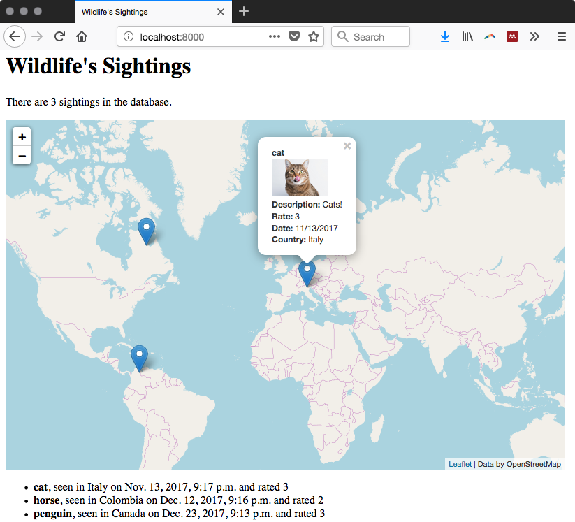
You created an HTML front page for the web application you developed in the previous recipe. The HTML is dynamically created using the Django template language (https://docs.djangoproject.com/en/dev/topics/templates/) and the map was implemented with the Leaflet JavaScript library.
The Django template language uses the response from the home view to generate a list of all of the sightings in the system.
The map was created using Leaflet. First, an OpenStreetMap layer was used as a base map. Then, using jQuery, you fed a GeoJSON layer that displays all of the features generated by the get_geojson view. You associated a popup with the layer that opens every time the user clicks on a sighting entity. The popup displays the main information for that sighting, including a picture of the sighted animal.
For this recipe, we will use the way points dataset from Chapter 3, Working with Vector Data – The Basics. Refer to the script in the recipe named Working with GPS data to learn how to import .gpx files tracks into PostGIS. You will also need a Mapbox token; for this, go to their site (https://www.mapbox.com) and sign up for one.
ogr2ogr -f GeoJSON tracks.json \
"PG:host=localhost dbname=postgis_cookbook user=me" \
-sql "select * from chp03.tracks
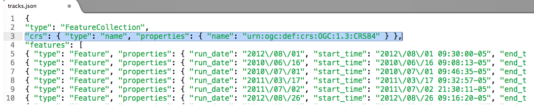
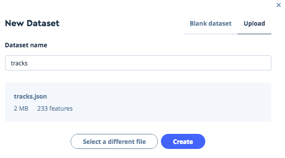

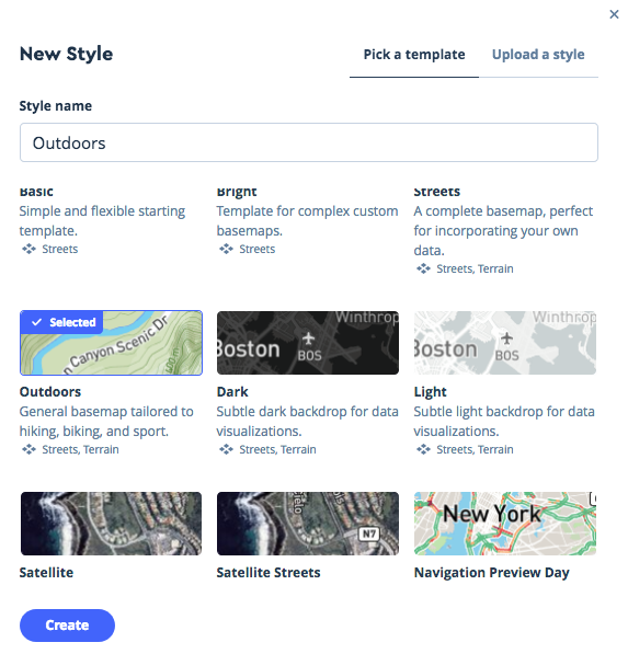
<script src='https://api.mapbox.com/mapbox-gl-js
/v0.42.0/mapbox-gl.js'></script>
<link href='https://api.mapbox.com/mapbox-gl-js
/v0.42.0/mapbox-gl.css' rel='stylesheet' />
<div id='map' style='width: 800px; height: 600px;'></div>
<script>
mapboxgl.accessToken = YOUR_TOKEN';
var map = new mapboxgl.Map({
container: 'map',
style: 'YOUR_STYLE_URL'
});
// Add zoom and rotation controls to the map.
map.addControl(new mapboxgl.NavigationControl());
</script>
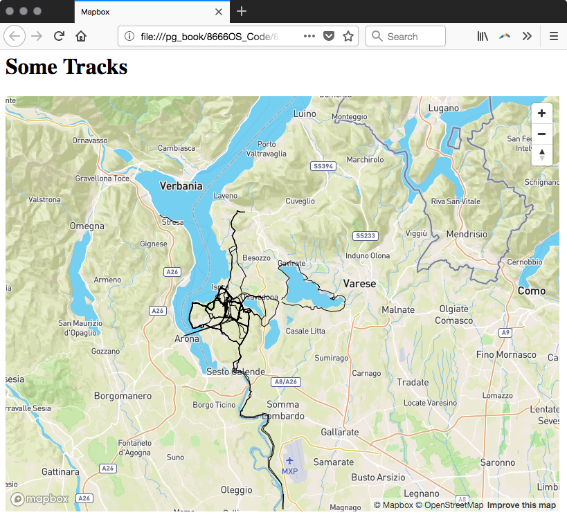
To quickly publish and visualize data in a webGIS, you can use the Mapbox API to create beautiful maps with your own data; you will have to keep a GeoJSON format and not exceed the offered bandwidth capacity. In this recipe, you've learned how to export your PostGIS data to publish it in Mapbox as a JS.
In this chapter, we will cover the following recipes:
Unlike prior chapters, this chapter does not discuss the capabilities or applications of PostGIS. Instead, it focuses on the techniques for organizing the database, improving the query performance, and ensuring the long-term viability of the spatial data.
These techniques are frequently ignored by most PostGIS users until it is too late - for example, when data has already been lost because of users' actions or the performance has already decreased as the volume of data or number of users increased.
Such neglect is often due to the amount of time required to learn about each technique, as well as the time it takes implement them. This chapter attempts to demonstrate each technique in a distilled manner that minimizes the learning curve and maximizes the benefits.
One of the most important things to consider when creating and using a database is how to organize the data. The layout should be decided when you first establish the database. The layout can be decided on or changed at a later date, but this is almost guaranteed to be a tedious, if not difficult, task. If it is never decided on, a database will become disorganized over time and introduce significant hurdles when upgrading components or running backups.
By default, a new PostgreSQL database has only one schema - namely, public. Most users place all the data (their own and third-party modules, such as PostGIS) in the public schema. Doing so mixes different information from various origins. An easy method with which to separate the information is by using schemas. This enables us to use one schema for our data and a separate schema for everything else.
In this recipe, we will create a database and install PostGIS in its own schema. We will also load some geometries and rasters for future use by other recipes in this chapter.
The following are the two methods to create a PostGIS-enabled database:
The CREATE EXTENSION method is available if you are running PostgreSQL 9.1 or a later version and is the recommended method for installing PostGIS:
Carry out the following steps to create and organize a database:
CREATE DATABASE chapter10;
CREATE SCHEMA postgis;
CREATE EXTENSION postgis WITH SCHEMA postgis;
The WITH SCHEMA clause of the CREATE EXTENSION statement instructs PostgreSQL to install PostGIS and its objects in the postgis schema.
> psql -U me -d chapter10
> chapter10=# SET search_path = public, postgis;
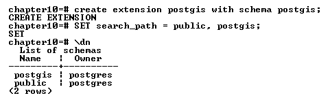
Verify the list of relations in the schema, which should include all the ones created by the extension:
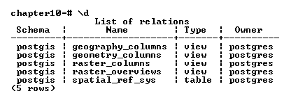
If you are using pgAdmin or a similar database system, you can also check on the graphical interface whether the schemas, views, and table were created successfully.
The SET statement instructs PostgreSQL to consider the public and postgis schemas when processing any SQL statements from our client connection. Without the SET statement, the \d command will not return any relation from the postgis schema.
ALTER DATABASE chapter10 SET search_path = public, postgis;
All future connections and queries to chapter10 will result in PostgreSQL automatically using both public and postgis schemas.
Note: It may be the case that, for Windows users, this option may not work well; in version 9.6.7 it worked but not in version 9.6.3. If it does not work, you may need to clearly define the search_path on every command. Both versions are provided.
> raster2pgsql -s 4322 -t 100x100 -I -F -C -Y
C:\postgis_cookbook\data\chap5
\PRISM\ PRISM_tmin_provisional_4kmM2_201703_asc.asc
prism | psql -d chapter10 -U me
Then, define the search path:
> raster2pgsql -s 4322 -t 100x100 -I -F -C -Y
C\:postgis_cookbook\data\chap5
\PRISM\PRISM_tmin_provisional_4kmM2_201703_asc.asc
prism | psql "dbname=chapter10 options=--search_path=postgis" me
ALTER TABLE postgis.prism ADD COLUMN month_year DATE;
UPDATE postgis.prism SET month_year = (
SUBSTRING(split_part(filename, '_', 5), 0, 5) || '-' ||
SUBSTRING(split_part(filename, '_', 5), 5, 4) || '-01'
) :: DATE;
> shp2pgsql -s 3310 -I
C\:postgis_cookbook\data\chap5\SFPoly\sfpoly.shp sfpoly |
psql -d chapter10 -U me
Then, define the search path:
> shp2pgsql -s 3310 -I
C\:postgis_cookbook\data\chap5\SFPoly\sfpoly.shp
sfpoly | psql "dbname=chapter10 options=--search_path=postgis" me
> mkdir C:\postgis_cookbook\data\chap10
> cp -r /path/to/book_dataset/chap10
C\:postgis_cookbook\data\chap10
We will use the shapefiles for California schools and police stations provided by the USEIT program at the University of Southern California. Import the shapefiles by executing the following commands; use the spatial index flag -I only for the police stations shapefile:
> shp2pgsql -s 4269 -I
C\:postgis_cookbook\data\chap10\CAEmergencyFacilities\CA_police.shp
capolice | psql -d chapter10 -U me
Then, define the search path:
> shp2pgsql -s 4269 C\:postgis_cookbook\data\chap10
\CAEmergencyFacilities\CA_schools.shp
caschools | psql -d chapter10 -U me
Then, define the search path:
shp2pgsql -s 4269 -I C\:postgis_cookbook\data\chap10
\CAEmergencyFacilities\CA_schools.shp
caschools | psql "dbname=chapter10 options=--search_path=postgis"
me shp2pgsql -s 4269 -I
C\:postgis_cookbook\data\chap10\CAEmergencyFacilities\CA_police.shp
capolice | psql "dbname=chapter10 options=--search_path=postgis" me
In this recipe, we created a new database and installed PostGIS in its own schema. We kept the PostGIS objects separate from our geometries and rasters without installing PostGIS in the public schema. This separation keeps the public schema tidy and reduces the accidental modification or deletion of the PostGIS objects. If the definition of the search path did not work, then use the explicit definition of the schema in all the commands, as shown.
In the following recipes, we will see that our decision to install PostGIS in its own schema results in fewer problems when maintaining the database.
PostgreSQL provides a fine-grained privilege system that dictates who can use a particular set of data and how that set of data can be accessed by an approved user. Because of its granular nature, creating an effective set of privileges can be confusing, and may result in undesired behavior. There are different levels of access that can be provided, from controlling who can connect to the database server itself, to who can query a view, to who can execute a PostGIS function.
The challenges of establishing a good set of privileges can be minimized by thinking of the database as an onion. The outermost layer has generic rules and each layer inward applies rules that are more specific than the last. An example of this is a company's database server that only the company's network can access.
Only one of the company's divisions can access database A, which contains a schema for each department. Within one schema, all users can run the SELECT queries against views, but only specific users can add, update, or delete records from tables.
In PostgreSQL, users and groups are known as roles. A role can be parent to other roles that are themselves parents to even more roles.
In this recipe, we focus on establishing the best set of privileges for the postgis schema created in the previous recipe. With the right selection of privileges, we can control who can use the contents of and apply operations to a geometry, geography, or raster column.
One aspect worth mentioning is that the owner of a database object (such as the database itself, a schema, or a table) always has full control over that object. Unless someone changes the owner, the user who created the database object is typically the owner of the object.
Again, when tested in Windows, the functionalities regarding the granting of permission worked on version 9.6.7 and did not work in version 9.6.3.
In the preceding recipe, we imported several rasters and shapefiles to their respective tables. By default, access to those tables is restricted to only the user who performed the import operation, also known as the owner. The following steps permit other users to access those tables:
CREATE ROLE group1 NOLOGIN;
CREATE ROLE group2 NOLOGIN;
CREATE ROLE user1 LOGIN PASSWORD 'pass1' IN ROLE group1;
CREATE ROLE user2 LOGIN PASSWORD 'pass2' IN ROLE group1;
CREATE ROLE user3 LOGIN PASSWORD 'pass3' IN ROLE group2;
The first two CREATE ROLE statements create the groups group1 and group2. The last three CREATE ROLE statements create three users, with the user1 and user2 users assigned to group1 and the user3 user assigned to group2.
GRANT CONNECT, TEMP ON DATABASE chapter10 TO GROUP group1;
GRANT ALL ON DATABASE chapter10 TO GROUP group2;
> psql -U me -d chapter10
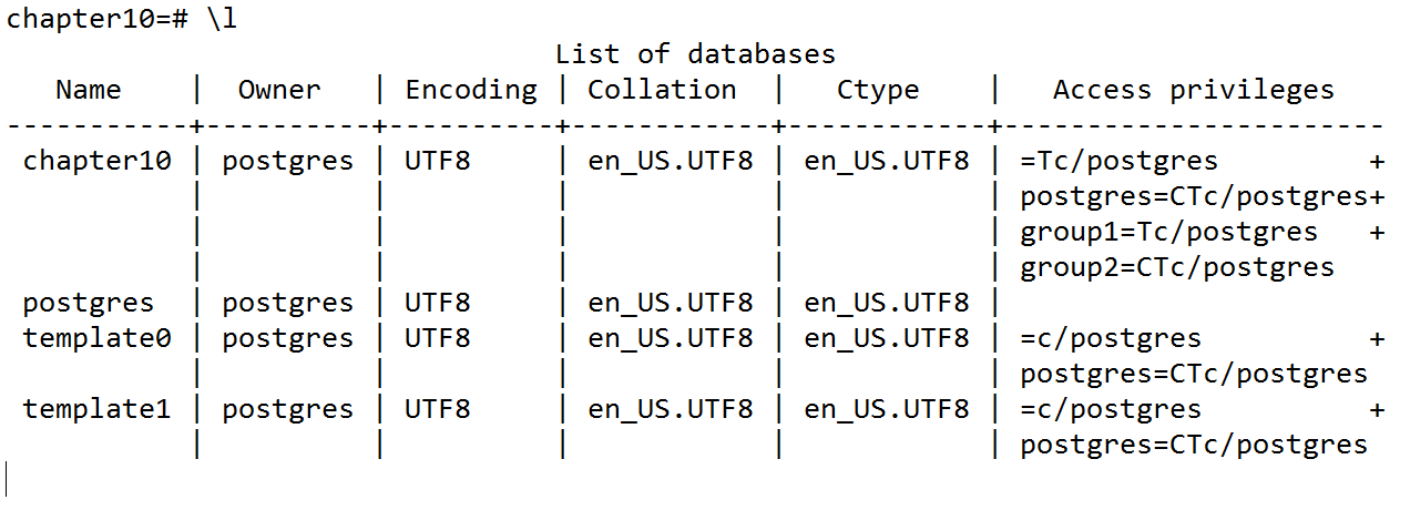
As you can see, group1 and group2 are present in the Access privileges column of the chapter10 database:
group1=Tc/postgres
group2=CTc/postgres
=Tc/postgres
Unlike the privilege listings for group1 and group2, this listing has no value before the equal sign (=). This listing is for the special metagroup public, which is built into PostgreSQL and to which all users and groups automatically belong.
REVOKE ALL ON DATABASE chapter10 FROM public;
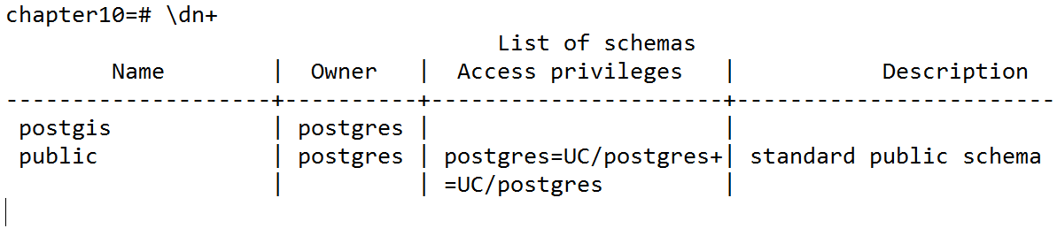
GRANT USAGE ON SCHEMA postgis TO group1, group2;
We generally do not want to grant the CREATE privilege in the postgis schema to any user or group. New objects (such as functions, views, and tables) should not be added to the postgis schema.
GRANT USAGE ON SCHEMA postgis TO public;
If you want to revoke this privilege, use the following command:
REVOKE USAGE ON SCHEMA postgis FROM public;
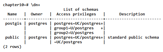
Granting the USAGE privilege to a schema does not allow the granted users and groups to use any objects in the schema. The USAGE privilege only permits the users and groups to view the schema's child objects. Each child object has its own set of privileges, which we establish in the remaining steps.
PostGIS comes with more than 1,000 functions. It would be unreasonable to individually set privileges for each of those functions. Instead, we grant the EXECUTE privilege to the metagroup public and then grant and/or revoke privileges to specific functions, such as management functions.
GRANT EXECUTE ON ALL FUNCTIONS IN SCHEMA postgis TO public;
REVOKE ALL ON FUNCTION postgis_full_version() FROM public;
If there are problems accessing the functions on the postgis schema, use the following command:
REVOKE ALL ON FUNCTION postgis.postgis_full_version() FROM public;
The GRANT and REVOKE statements do not differentiate between tables and views, so care must be taken to ensure that the applied privileges are appropriate for the object.
GRANT SELECT, REFERENCES, TRIGGER
ON ALL TABLES IN SCHEMA postgis TO public;
GRANT INSERT ON spatial_ref_sys TO group1;
Groups and users that are not part of group1 (such as group2) can only use the SELECT statements on spatial_ref_sys. Groups and users that are part of group1 can now use the INSERT statement to add new spatial reference systems.
GRANT UPDATE, DELETE ON spatial_ref_sys TO user2;
> psql -d chapter10 -u user3
chapter10=# SELECT count(*) FROM spatial_ref_sys;
Of if the schema need to be defined, use the following sentence:
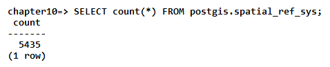
chapter10=# INSERT INTO spatial_ref_sys
VALUES (99999, 'test', 99999, '', ''); ERROR: permission denied for relation spatial_ref_sys
chapter10=# UPDATE spatial_ref_sys SET srtext = 'Lorum ipsum';
ERROR: permission denied for relation spatial_ref_sys
chapter10=# SELECT postgis_full_version();
ERROR: permission denied for function postgis_full_version
In this recipe, we granted and revoked privileges based on the group or user, with security increasing as a group or user descends into the database. This resulted in group1 and group2 being able to connect to the chapter10 database and use objects found in the postgis schema. group1 could also insert new records into the spatial_ref_sys table. Only user2 was permitted to update or delete the records of spatial_ref_sys.
The GRANT and REVOKE statements used in this recipe work, but they can be tedious to use with a command-line utility, such as psql. Instead, use a graphical tool, such as pgAdmin, that provides a grant wizard. Such tools also make it easier to check the behavior of the database after granting and revoking privileges.
For additional practice, set up the privileges on the public schema and child objects so that, although group1 and group2 will be able to run the SELECT queries on the tables, only group2 will be able to use the INSERT statement on the caschools table. You will also want to make sure that an INSERT statement executed by a user of group2 actually works.
Maintaining functional backups of your data and work is probably the least appreciated, yet the most important thing you can do to improve your productivity (and stress levels). You may think that you don't need to have backups of your PostGIS database because you have the original data imported to the database, but do you remember all the work you did to develop the final product? How about the intermediary products? Even if you remember every step in the process, how much time will it take to create the intermediary and final products?
If any of these questions gives you pause, you need to create a backup for your data. Fortunately, PostgreSQL makes the backup process painless, or at least less painful than the alternatives.
In this recipe, we use PostgreSQL's pg_dump utility. The pg_dump utility ensures that the data being backed up is consistent, even if it is currently in use.
Use the following steps to back up a database:
> pg_dump -f chapter10.backup -F custom chapter10
We use the -f flag to specify that the backup should be placed in the chapter10.backup file. We also use the -F flag to set the format of the backup output as custom - the most flexible and compressed of pg_dump's output formats by default.
> pg_restore -f chapter10.sql chapter10.backup
After creating a backup, it is good practice to make sure that the backup is valid. We do so with the pg_restore PostgreSQL tool. The -f flag instructs pg_restore to emit the restored output to a file instead of a database. The emitted output comprises standard SQL statements.
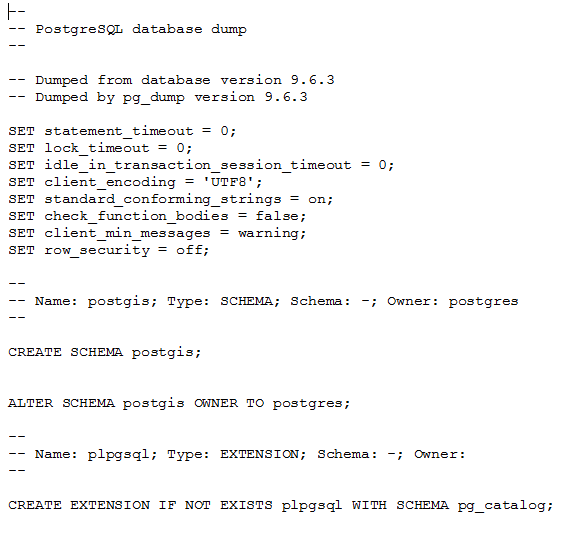
And the files continue to show information about tables, sequences, and so on:
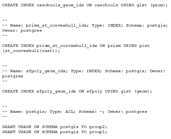
> pg_restore -f chapter10_public.sql -n public chapter10.backup
If you compare chapter10_public.sql to the chapter10.sql file exported in the preceding step, you will see that the postgis schema is not restored.
As you can see, backing up your database is easy in PostgreSQL. Unfortunately, backups are meaningless if they are not performed on a regular schedule. If the database is lost or corrupted, any work done since the last backup is also lost. It is recommended that you perform backups at intervals that minimize the amount of work lost. The ideal interval will depend on the frequency of changes made to the database.
The pg_dump utility can be scheduled to run at regular intervals by adding a job to the operating system's task scheduler; the instructions for doing this are available in the PostgreSQL wiki at http://wiki.postgresql.org/wiki/Automated_Backup_on_Windows and http://wiki.postgresql.org/wiki/Automated_Backup_on_Linux.
The pg_dump utility is not adequate for all situations. If you have a database undergoing constant changes or that is larger than a few tens of gigabytes, you will need a backup mechanism far more robust than that discussed in this recipe. Information regarding these robust mechanisms can be found in the PostgreSQL documentation at http://www.postgresql.org/docs/current/static/backup.html.
The following are several third-party backup tools available for establishing robust and advanced backup schemes:
A database index is very much like the index of a book (such as this one). While a book's index indicates the pages on which a word is present, a database column index indicates the rows in a table that contain a searched-for value. Just as a book's index does not indicate exactly where on the page a word is located, the database index may not be able to denote the exact location of the searched-for value in a row's column.
PostgreSQL has several types of index, such as B-Tree, Hash, GIST, SP-GIST, and GIN. All of these index types are designed to help queries find matching rows faster. What makes the indices different are the underlying algorithms. Generally, to keep things simple, almost all PostgreSQL indexes are of the B-Tree type. PostGIS (spatial) indices are of the GIST type.
Geometries, geographies, and rasters are all large, complex objects, and relating to or among these objects takes time. Spatial indices are added to the PostGIS data types to improve search performance. The performance improvement comes not from comparing actual, potentially complex, spatial objects, but rather the simple bounding boxes of those objects.
For this recipe, psql will be used as follows to time the queries:
> psql -U me -d chapter10 chapter10=# \timing on
We will use the caschools and sfpoly tables loaded in this chapter's first recipe.
The best way to see how a query can be affected by an index is by running the query before and after the addition of an index. In this recipe, in order to avoid the need to define the schema, all the tables are assumed to be on the public schema. The following steps will guide you through the process of optimizing a query with an index:
SELECT schoolid FROM caschools sc JOIN sfpoly sf
ON ST_Intersects(sf.geom, ST_Transform(sc.geom, 3310));
Time: 136.643 ms
Time: 140.863 ms
Time: 135.859 ms
EXPLAIN ANALYZE
SELECT schoolid FROM caschools sc JOIN sfpoly sf
ON ST_Intersects(sf.geom, ST_Transform(sc.geom, 3310));
Adding EXPLAIN ANALYZE before the query instructs PostgreSQL to return the actual plan used to execute the query, as follows:
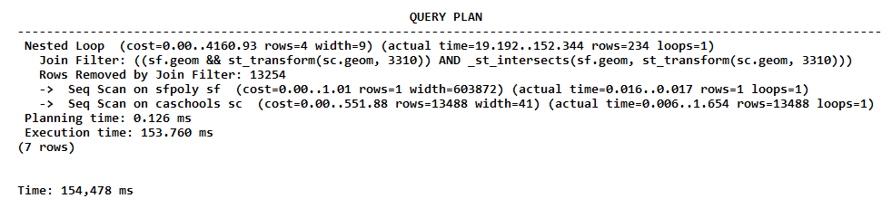
What is significant in the preceding QUERY PLAN is Join Filter, which has consumed most of the execution time. This may be happening because the caschools table does not have a spatial index on the geom column.
CREATE INDEX caschools_geom_idx ON caschools
USING gist (geom);
Time: 95.807 ms
Time: 101.626 ms
Time: 103.748 ms
The query did not run much faster with the spatial index. What happened? We need to check the QUERY PLAN.
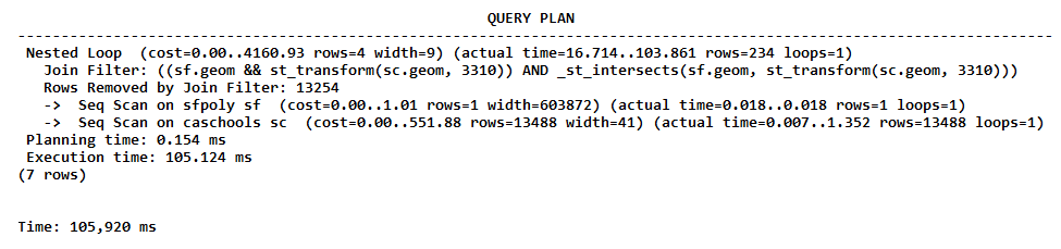
The QUERY PLAN table is the same as that found in step 4. The query is not using the spatial index. Why?
If you look at the query, we used ST_Transform() to reproject caschools.geom on the spatial reference system of sfpoly.geom. The ST_Transform() geometries used in the ST_Intersects() spatial test were in SRID 3310, but the geometries used for the caschools_geom_idx index were in SRID 4269. This difference in spatial reference systems prevented the use of the index in the query.
CREATE INDEX caschools_geom_3310_idx ON caschools
USING gist (ST_Transform(geom, 3310));
Time: 63.359 ms
Time: 64.611 ms
Time: 56.485 ms
That's better! The duration of the process has decreased from about 135 ms to 60 ms.
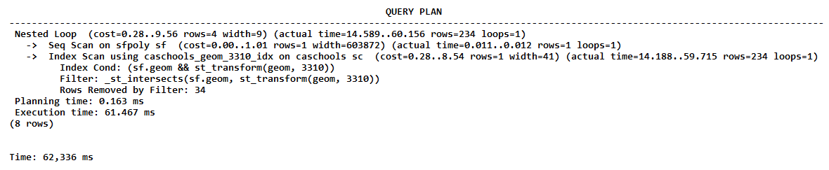
The plan shows that the query used the caschools_geom_3310_idx index. The Index Scan command was significantly faster than the previously used Join Filter command.
Database indices help us quickly and efficiently find the values we are interested in. Generally, a query using an index is faster than one that is not, but the performance improvement may not be to the degree found in this recipe.
Additional information about PostgreSQL and PostGIS indices can be found at the following links:
We will discuss query plans in greater detail in a later recipe in this chapter. By understanding query plans, it becomes possible to optimize the performance of deficient queries.
Most users stop optimizing the performance of a table after adding the appropriate indices. This usually happens because the performance reaches a point where it is good enough. But what if the table has millions or billions of records? This amount of information may not fit in the database server's RAM, thereby forcing hard drive access. Generally, table records are stored sequentially on the hard drive. But the data being fetched for a query from the hard drive may be accessing many different parts of the hard drive. Having to access different parts of a hard drive is a known performance limitation.
To mitigate hard drive performance issues, a database table can have its records reordered on the hard drive so that similar record data is stored next to or near each other. The reordering of a database table is known as clustering and is used with the CLUSTER statement in PostgreSQL.
We will use the California schools (caschools) and San Francisco boundaries (sfpoly) tables for this recipe. If neither table is available, refer to the first recipe of this chapter.
The psql utility will be used for this recipe's queries, as shown here:
> psql -U me -d chapter10 chapter10=# \timing on
Use the following steps to cluster a table:
SELECT schoolid FROM caschools sc JOIN sfpoly sf
ON ST_Intersects(sf.geom, ST_Transform(sc.geom, 3310));
Time: 80.746 ms
Time: 80.172 ms
Time: 80.004 ms
CLUSTER caschools USING caschools_geom_3310_idx;
Time: 57.880 ms
Time: 55.939 ms
Time: 53.107 ms
The performance improvements were not significant.
Using the CLUSTER statement on the caschools table did not result in a significant performance boost. The lesson here is that, despite the fact that the data is physically reordered based on the index information in order to optimize searching, there is no guarantee that query performance will improve on a clustered table. Clustering should be reserved for tables with many large records only after adding the appropriate indices to and optimizing queries for the tables in question.
When an SQL query is received, PostgreSQL runs the query through its planner to decide the best execution plan. The best execution plan generally results in the fastest query performance. Though the planner usually makes the correct choices, on occasion, a specific query will have a suboptimal execution plan.
For these situations, the following are several things that can be done to change the behavior of the PostgreSQL planner:
Adding indices (the first bullet point) is discussed in a separate recipe found in this chapter. Updating statistics (the second point) is generally done automatically by PostgreSQL after a certain amount of table activity, but the statistics can be manually updated using the ANALYZE statement. Changing the database layout and the query planner's configuration (the fourth and fifth bullet point, respectively) are advanced operations used only when the first three points have already been attempted and, thus, will not be discussed further.
This recipe only discusses the third option - that is, optimizing performance by rewriting SQL queries.
For this recipe, we will find the nearest police station to every school and the distance in meters between each school in San Francisco and its nearest station; we will attempt to do this as fast as possible. This will require us to rewrite our query many times to be more efficient and take advantage of the new PostgreSQL capabilities. For this recipe, ensure that you also include the capolice table.
The following steps will guide you through the iterative process required to improve query performance:
SELECT
di.school,
police_address,
distance
FROM ( -- for each school, get the minimum distance to a
-- police station
SELECT
gid,
school,
min(distance) AS distance
FROM ( -- get distance between every school and every police
-- station in San Francisco
SELECT
sc.gid,
sc.name AS school,
po.address AS police_address,
ST_Distance(po.geom_3310, sc.geom_3310) AS distance
FROM ( -- get schools in San Francisco
SELECT
ca.gid,
ca.name,
ST_Transform(ca.geom, 3310) AS geom_3310
FROM sfpoly sf
JOIN caschools ca
ON ST_Intersects(sf.geom, ST_Transform(ca.geom, 3310))
) sc
CROSS JOIN ( -- get police stations in San Francisco
SELECT
ca.address,
ST_Transform(ca.geom, 3310) AS geom_3310
FROM sfpoly sf
JOIN capolice ca
ON ST_Intersects(sf.geom, ST_Transform(ca.geom, 3310))
) po ORDER BY 1, 2, 4
) scpo
GROUP BY 1, 2
ORDER BY 2
) di JOIN ( -- for each school, collect the police station
-- addresses ordered by distance
SELECT
gid,
school,
(array_agg(police_address))[1] AS police_address
FROM (-- get distance between every school and
every police station in San Francisco
SELECT
sc.gid,
sc.name AS school,
po.address AS police_address,
ST_Distance(po.geom_3310, sc.geom_3310) AS distance
FROM ( -- get schools in San Francisco
SELECT
ca.gid,
ca.name,
ST_Transform(ca.geom, 3310) AS geom_3310
FROM sfpoly sf
JOIN caschools ca
ON ST_Intersects(sf.geom, ST_Transform(ca.geom, 3310))
) sc
CROSS JOIN ( -- get police stations in San Francisco
SELECT
ca.address,
ST_Transform(ca.geom, 3310) AS geom_3310
FROM sfpoly sf JOIN capolice ca
ON ST_Intersects(sf.geom, ST_Transform(ca.geom, 3310))
) po
ORDER BY 1, 2, 4
) scpo
GROUP BY 1, 2
ORDER BY 2
) po
ON di.gid = po.gid
ORDER BY di.school;
Note: the time may vary substantially between experiments, depending on the machine configuration, database usage, and so on. However, the changes in the duration of the experiments will be noticeable and should follow the same improvement ratio presented in this section.
The query output looks as follows:
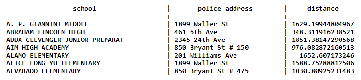
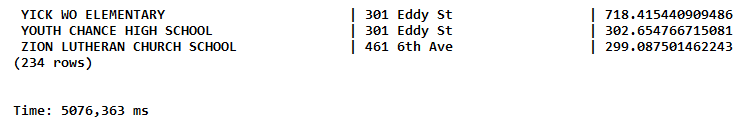
Time: 5076.363 ms
Time: 4974.282 ms
Time: 5027.721 ms
WITH scpo AS ( -- get distance between every school and every
-- police station in San Francisco SELECT sc.gid, sc.name AS school, po.address AS police_address, ST_Distance(po.geom_3310, sc.geom_3310) AS distance
FROM ( -- get schools in San Francisco SELECT ca.*, ST_Transform(ca.geom, 3310) AS geom_3310 FROM sfpoly sf JOIN caschools ca ON ST_Intersects(sf.geom, ST_Transform(ca.geom, 3310)) ) sc CROSS JOIN ( -- get police stations in San Francisco
SELECT ca.*, ST_Transform(ca.geom, 3310) AS geom_3310 FROM sfpoly sf JOIN capolice ca ON ST_Intersects(sf.geom, ST_Transform(ca.geom, 3310)) ) po ORDER BY 1, 2, 4 ) SELECT di.school, police_address, distance FROM ( -- for each school, get the minimum distance to a -- police station SELECT gid, school, min(distance) AS distance
FROM scpo GROUP BY 1, 2 ORDER BY 2 ) di JOIN ( -- for each school, collect the police station
-- addresses ordered by distance SELECT gid, school, (array_agg(police_address))[1] AS police_address FROM scpo GROUP BY 1, 2 ORDER BY 2 ) po ON di.gid = po.gid ORDER BY 1;
Time: 2803.923 ms
Time: 2798.105 ms
Time: 2796.481 ms
The execution times went from more than 5 seconds to less than 3 seconds.
WITH scpo AS ( -- get distance between every school and every
-- police station in San Francisco
SELECT sc.name AS school, po.address AS police_address, ST_Distance(po.geom_3310, sc.geom_3310) AS distance
FROM ( -- get schools in San Francisco SELECT ca.name, ST_Transform(ca.geom, 3310) AS geom_3310 FROM sfpoly sf JOIN caschools ca ON ST_Intersects(sf.geom, ST_Transform(ca.geom, 3310))
) sc CROSS JOIN ( -- get police stations in San Francisco SELECT ca.address, ST_Transform(ca.geom, 3310) AS geom_3310 FROM sfpoly sf JOIN capolice ca ON ST_Intersects(sf.geom, ST_Transform(ca.geom, 3310)) ) po ORDER BY 1, 3, 2 ) SELECT DISTINCT school, first_value(police_address)
OVER (PARTITION BY school ORDER BY distance), first_value(distance)
OVER (PARTITION BY school ORDER BY distance) FROM scpo ORDER BY 1;
Time: 1261.473 ms
Time: 1217.843 ms
Time: 1215.086 ms
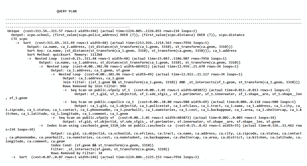
...
-> Nested Loop (cost=0.15..311.48 rows=1 width=48)
(actual time=15.047..1186.907 rows=7956 loops=1)
Output: ca.name, ca_1.address,
st_distance(st_transform(ca_1.geom, 3310),
st_transform(ca.geom, 3310))
WITH sc AS ( -- get schools in San Francisco
SELECT
ca.gid,
ca.name,
ca.geom
FROM sfpoly sf
JOIN caschools ca
ON ST_Intersects(sf.geom, ST_Transform(ca.geom, 3310))
), po AS ( -- get police stations in San Francisco
SELECT
ca.gid,
ca.address,
ca.geom
FROM sfpoly sf
JOIN capolice ca
ON ST_Intersects(sf.geom, ST_Transform(ca.geom, 3310))
)
SELECT
school,
police_address,
ST_Distance(ST_Transform(school_geom, 3310),
ST_Transform(police_geom, 3310)) AS distance
FROM ( -- for each school, number and order the police
-- stations by how close each station is to the school
SELECT
ROW_NUMBER() OVER (
PARTITION BY sc.gid ORDER BY sc.geom <-> po.geom
) AS r,
sc.name AS school,
sc.geom AS school_geom,
po.address AS police_address,
po.geom AS police_geom
FROM sc
CROSS JOIN po
) scpo
WHERE r < 2
ORDER BY 1;
Time: 83.002 ms
Time: 82.586 ms
Time: 83.327 ms
Wow! Using indexed nearest-neighbor searches with the <-> operator, we reduced our initial query from one second to less than a tenth of a second.
In this recipe, we optimized a query that users may commonly encounter while using PostGIS. We started by taking advantage of the PostgreSQL capabilities to improve the performance and syntax of our query. When performance could no longer improve, we ran EXPLAIN ANALYZE VERBOSE to find out what was consuming most of the query-execution time. We learned that the ST_Distance() function consumed the most time from the execution plan. We finally used the <-> operator of PostgreSQL 9.1 to dramatically improve the query-execution time to under a second.
The output of EXPLAIN ANALYZE VERBOSE used in this recipe is not easy to understand. For complex queries, it is recommended that you use the visual output in pgAdmin (discussed in a separate chapter's recipe) or the color coding provided by the http://explain.depesz.com/ web service, as shown in the following screenshot:
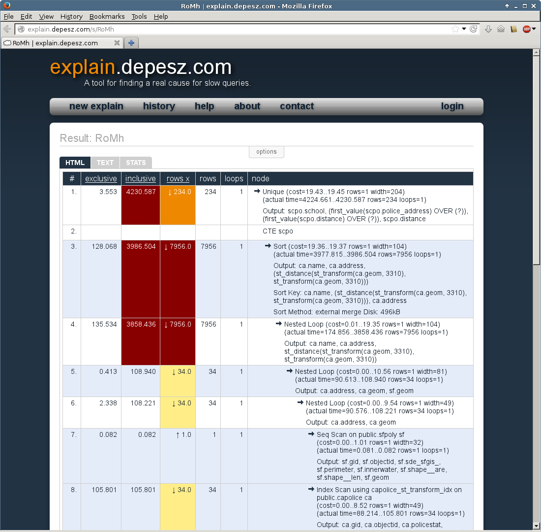
At some point, user databases need to be migrated to a different server. This need for server migration could be due to new hardware or a database-server software upgrade.
The following are the three methods available for migrating a database:
In this recipe, we will use the dump and restore methods to move user data to a new database with a new PostGIS installation. Unlike the other methods, this method is the most foolproof, works in all situations, and stores a backup in case things don't work as expected.
As mentioned before, creating a schema specifically to work with PostGIS may not work properly for Windows users. Working on the public schema is an option in order to test the results.
On the command line, perform the following steps:
> pg_dump -U me -f chapter10.backup -F custom chapter10
> psql -d postgres -U me
postgres=# CREATE DATABASE new10;
postgres=# \c new10
new10=# CREATE SCHEMA postgis;
new10=# CREATE EXTENSION postgis WITH SCHEMA postgis;
new10=# ALTER DATABASE new10 SET search_path = public, postgis;
> pg_restore -U me -d new10 --schema=public chapter10.backup
pg_restore: [archiver (db)] Error while PROCESSING TOC:
pg_restore: [archiver (db)] Error from TOC entry 3781; 03496229
TABLE DATA prism postgres
pg_restore: [archiver (db)] COPY failed for table "prism":
ERROR: function st_bandmetadata(postgis.raster, integer[])
does not exist
LINE 1: SELECT array_agg(pixeltype)::text[]
FROM st_bandmetadata($1...
We have now installed PostGIS in the postgis schema, but the database server can't find the ST_BandMetadata() function. If a function cannot be found, it is usually an issue with search_path. We will fix this issue in the next step.
pg_restore -f chapter10.sql --schema=public chapter10.backup
SET search_path = public, pg_catalog;
SET search_path = public, postgis, pg_catalog;
> psql -U me -d new10 -f chapter10.sql
This procedure is essentially the standard PostgreSQL backup and restore cycle. It may not be simple, but has the benefit of being accessible in terms of the tools used and the control available in each step of the process. Though the other migration methods may be convenient, they typically require faith in an opaque process or the installation of additional software.
The reality of the world is that, given enough time, everything will break. This includes the hardware and software of computers running PostgreSQL. To protect data in PostgreSQL from corruption or loss, backups are taken using tools such as pg_dump. However, restoring a database backup can take a very long time, during which users cannot use the database.
When downtime must be kept to a minimum or is not acceptable, one or more standby servers are used to compensate for the failed primary PostgreSQL server. The data on the standby server is kept in sync with the primary PostgreSQL server by streaming data as frequently as possible.
In addition, you are strongly discouraged from trying to mix different PostgreSQL versions. Primary and standby servers must run the same PostgreSQL version.
In this recipe, we will use the streaming replication capability introduced in PostgreSQL 9.X. This recipe will use one server with two parallel PostgreSQL installations instead of the typical two or more servers, each with one PostgreSQL installation. We will use two new database clusters in order to keep things simple.
Use the following steps to replicate a PostGIS database:
> mkdir postgis_cookbook/db
> mkdir postgis_cookbook/db/primary
> mkdir postgis_cookbook/db/standby
> cd postgis_cookbook/db
> initdb --encoding=utf8 --locale=en_US.utf-8 -U me -D primary
> initdb --encoding=utf8 --locale=en_US.utf-8 -U me -D standby
> mkdir postgis_cookbook/db/primary/archive
> mkdir postgis_cookbook/db/standby/archive
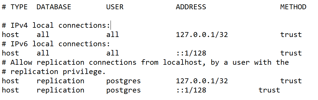
port = 5433
wal_level = hot_standby
max_wal_senders = 5
wal_keep_segments = 32
archive_mode = on
archive_command = 'copy "%p"
"C:\\postgis_cookbook\\db\\primary\\archive\\%f"' # for Windows
A relative location could also be used:
archive_command = 'copy "%p" "archive\\%f" "%p"'
When using Linux or macOS type instead:
archive_command = 'cp %p archive\/%f'
> pg_ctl start -D primary -l primary\postgres.log
> notepad exclude.txt
postmaster.pid
pg_xlog
> psql -p 5433 -U me -c "SELECT pg_start_backup('base_backup', true)"
> xcopy primary\* standby\ /e /exclude:primary\exclude.txt
> psql -p 5433 -U me -c "SELECT pg_stop_backup()"
port = 5434
hot_standby = on
archive_command = 'copy "%p"
"C:\\postgis_cookbook\\db\\standby\\archive\\%f"' # for Windows
A relative location could also be used:
archive_command = 'copy ".\\archive\\%f" "%p"'
When using Linux or macOS type instead:
archive_command = 'cp %p archive\/%f'
> notepad standby\recovery.conf
For Linux or macOS:
> nano standby\recovery.conf
standby_mode = 'on'
primary_conninfo = 'port=5433 user=me'
restore_command = 'copy
"C:\\postgis_cookbook\\db\\standby\\archive\\%f" "%p"'
Or a relative location could be used also:
restore_command = 'copy ".\\archive\\%f" "%p"'
For Linux or macOS use:
restore_command = 'cp %p \archive\/%f"'
> pg_ctl start -U me -D standby -l standby\postgres.log
> psql -p 5433 -U me
postgres=# CREATE DATABASE test;
postgres=# \c test
test=# CREATE TABLE test AS SELECT 1 AS id, 'one'::text AS value;
> psql -p 5434 -U me
postgres=# \l
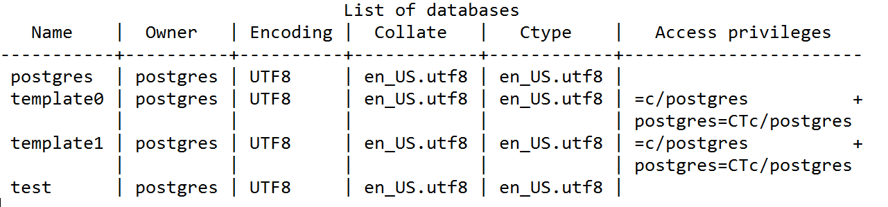
postgres=# \c test
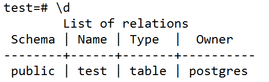
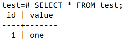
Congratulations! The streaming replication works.
As demonstrated in this recipe, the basic setup for streaming replication is straightforward. Changes made to the primary database server are quickly pushed to the standby database server.
There are third-party applications to help establish, administer, and maintain streaming replication on production servers. These applications permit complex replication strategies, including multimaster, multistandby, and proper failover. A few of these applications include the following:
Working with large datasets can be challenging for the database engine, especially when they are stored in a single table or in a single database. PostgreSQL offers an option to split the data into several external databases, with smaller tables, that work logically as one. Sharding allows distributing the load of storage and processing of a large dataset so that the impact of large local tables is reduced.
One of the most important issues to make it work is the definition of a function to classify and evenly distribute the data. Given that this function can be a geographical property, sharding can be applied to geospatial data.
In this recipe, we will use the postgres_fdw extension that allows the creation of foreign data wrappers, needed to access data stored in external PostgreSQL databases. In order to use this extension, we will need the combination of several concepts: server, foreign data wrapper, user mapping, foreign table and table inheritance. We will see them in action in this recipe, and you are welcome to explore them in detail on the PostgreSQL documentation.
We will use the fire hotspot dataset and the world country borders shapefile used in Chapter 1, Moving Data in and out of PostGIS, in order to distribute the records for the hotspot data based on a geographical criteria, we will create a new distributed version of the hotspot dataset.
We will use the postgis_cookbook database for this recipe.
If you did not follow the recipes in Chapter 1, Moving Data in and out of PostGIS, be sure to import the hotspots (Global_24h.csv) in PostGIS. The following steps explain how to do it with ogr2ogr (you should import the dataset in their original SRID, 4326, to make spatial operations faster):
> psql -d postgis_cookbook -U me
postgis_cookbook=# CREATE SCHEMA chp10;
postgis_cookbook =# CREATE TABLE chp10.hotspots_dist (id serial
PRIMARY KEY, the_geom public.geometry(Point,4326));
postgis_cookbook=# \q
> psql -U me
postgres=# CREATE DATABASE quad_NW;
CREATE DATABASE quad_NE;
CREATE DATABASE quad_SW;
CREATE DATABASE quad_SE;
postgres=# \c quad_NW;
quad_NW =# CREAT EXTENSION postgis;
quad_NW =# CREATE TABLE hotspots_quad_NW (
id serial PRIMARY KEY,
the_geom public.geometry(Point,4326)
);
quad_NW =# \c quad_NE;
quad_NE =# CREAT EXTENSION postgis;
quad_NE =# CREATE TABLE hotspots_quad_NE (
id serial PRIMARY KEY,
the_geom public.geometry(Point,4326)
);
quad_NW =# \c quad_SW;
quad_SW =# CREAT EXTENSION postgis;
quad_SW =# CREATE TABLE hotspots_quad_SW (
id serial PRIMARY KEY,
the_geom public.geometry(Point,4326)
);
quad_SW =# \c quad_SE;
quad_SE =# CREAT EXTENSION postgis;
quad_SE =# CREATE TABLE hotspots_quad_SE (
id serial PRIMARY KEY,
the_geom public.geometry(Point,4326)
);
quad_SE =# \q
<OGRVRTDataSource>
<OGRVRTLayer name="Global_24h">
<SrcDataSource>Global_24h.csv</SrcDataSource>
<GeometryType>wkbPoint</GeometryType>
<LayerSRS>EPSG:4326</LayerSRS>
<GeometryField encoding="PointFromColumns"
x="longitude" y="latitude"/>
</OGRVRTLayer>
</OGRVRTDataSource>
$ ogr2ogr -f PostgreSQL PG:"dbname='postgis_cookbook' user='me'
password='mypassword'" -lco SCHEMA=chp10 global_24h.vrt
-lco OVERWRITE=YES -lco GEOMETRY_NAME=the_geom -nln hotspots
postgis_cookbook =# CREATE EXTENSION postgres_fdw;
postgis_cookbook =# CREATE SERVER quad_NW
FOREIGN DATA WRAPPER postgres_fdw OPTIONS
(dbname 'quad_NW', host 'localhost', port '5432'); CREATE SERVER quad_SW FOREIGN DATA WRAPPER postgres_fdw OPTIONS
(dbname 'quad_SW', host 'localhost', port '5432'); CREATE SERVER quad_NE FOREIGN DATA WRAPPER postgres_fdw OPTIONS
(dbname 'quad_NE', host 'localhost', port '5432'); CREATE SERVER quad_SE FOREIGN DATA WRAPPER postgres_fdw OPTIONS
(dbname 'quad_SE', host 'localhost', port '5432');
postgis_cookbook =# CREATE USER MAPPING FOR POSTGRES SERVER quad_NW
OPTIONS (user 'remoteme1', password 'myPassremote1'); CREATE USER MAPPING FOR POSTGRES SERVER quad_SW
OPTIONS (user 'remoteme2', password 'myPassremote2'); CREATE USER MAPPING FOR POSTGRES SERVER quad_NE
OPTIONS (user 'remoteme3', password 'myPassremote3'); CREATE USER MAPPING FOR POSTGRES SERVER quad_SE
OPTIONS (user 'remoteme4', password 'myPassremote4');
postgis_cookbook =# CREATE FOREIGN TABLE hotspots_quad_NW ()
INHERITS (chp10.hotspots_dist) SERVER quad_NW
OPTIONS (table_name 'hotspots_quad_sw'); CREATE FOREIGN TABLE hotspots_quad_SW () INHERITS (chp10.hotspots_dist)
SERVER quad_SW OPTIONS (table_name 'hotspots_quad_sw'); CREATE FOREIGN TABLE hotspots_quad_NE () INHERITS (chp10.hotspots_dist)
SERVER quad_NE OPTIONS (table_name 'hotspots_quad_ne'); CREATE FOREIGN TABLE hotspots_quad_SE () INHERITS (chp10.hotspots_dist)
SERVER quad_SE OPTIONS (table_name 'hotspots_quad_se');
postgis_cookbook=# CREATE OR REPLACE
FUNCTION __trigger_users_before_insert() RETURNS trigger AS $__$
DECLARE
angle integer;
BEGIN
EXECUTE $$ select (st_azimuth(ST_geomfromtext('Point(0 0)',4326),
$1)
/(2*PI()))*360 $$ INTO angle
USING NEW.the_geom;
IF (angle >= 0 AND angle<90) THEN
EXECUTE $$
INSERT INTO hotspots_quad_ne (the_geom) VALUES ($1)
$$ USING
NEW.the_geom;
END IF;
IF (angle >= 90 AND angle <180) THEN
EXECUTE $$ INSERT INTO hotspots_quad_NW (the_geom) VALUES ($1)
$$ USING NEW.the_geom;
END IF;
IF (angle >= 180 AND angle <270) THEN
EXECUTE $$ INSERT INTO hotspots_quad_SW (the_geom) VALUES ($1)
$$ USING NEW.the_geom;
END IF;
IF (angle >= 270 AND angle <360) THEN
EXECUTE $$ INSERT INTO hotspots_quad_SE (the_geom) VALUES ($1)
$$ USING NEW.the_geom;
END IF;
RETURN null;
END;
$__$ LANGUAGE plpgsql;
CREATE TRIGGER users_before_insert
BEFORE INSERT ON chp10.hotspots_dist
FOR EACH ROW EXECUTE PROCEDURE __trigger_users_before_insert();
postgis_cookbook=# INSERT INTO CHP10.hotspots_dist (the_geom)
VALUES (0, st_geomfromtext('POINT (10 10)',4326));
INSERT INTO CHP10.hotspots_dist (the_geom)
VALUES ( st_geomfromtext('POINT (-10 10)',4326));
INSERT INTO CHP10.hotspots_dist (the_geom)
VALUES ( st_geomfromtext('POINT (-10 -10)',4326));
postgis_cookbook=# SELECT ST_ASTEXT(the_geom)
FROM CHP10.hotspots_dist;
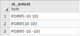
postgis_cookbook=# SELECT ST_ASTEXT(the_geom) FROM hotspots_quad_ne;
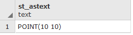
The remote databases only has the point that it should store, based on the trigger function defined earlier.
postgis_cookbook=# insert into CHP10.hotspots_dist
(the_geom, quadrant)
select the_geom, 0 as geom from chp10.hotspots;
postgis_cookbook=# SELECT ST_ASTEXT(the_geom)
FROM CHP10.hotspots_dist;
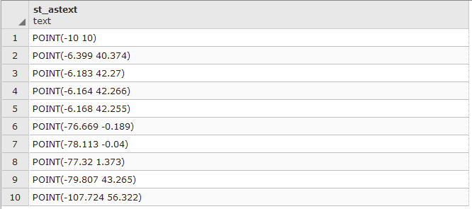
postgis_cookbook=# SELECT ST_ASTEXT(the_geom) FROM hotspots_quad_ne;
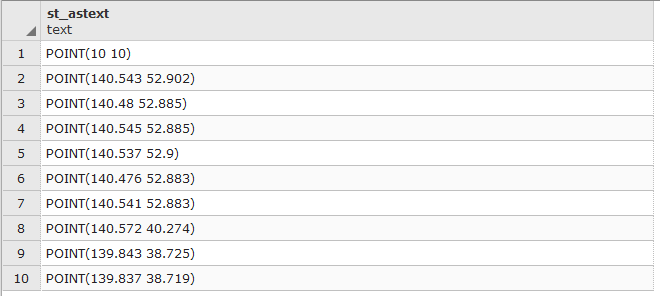
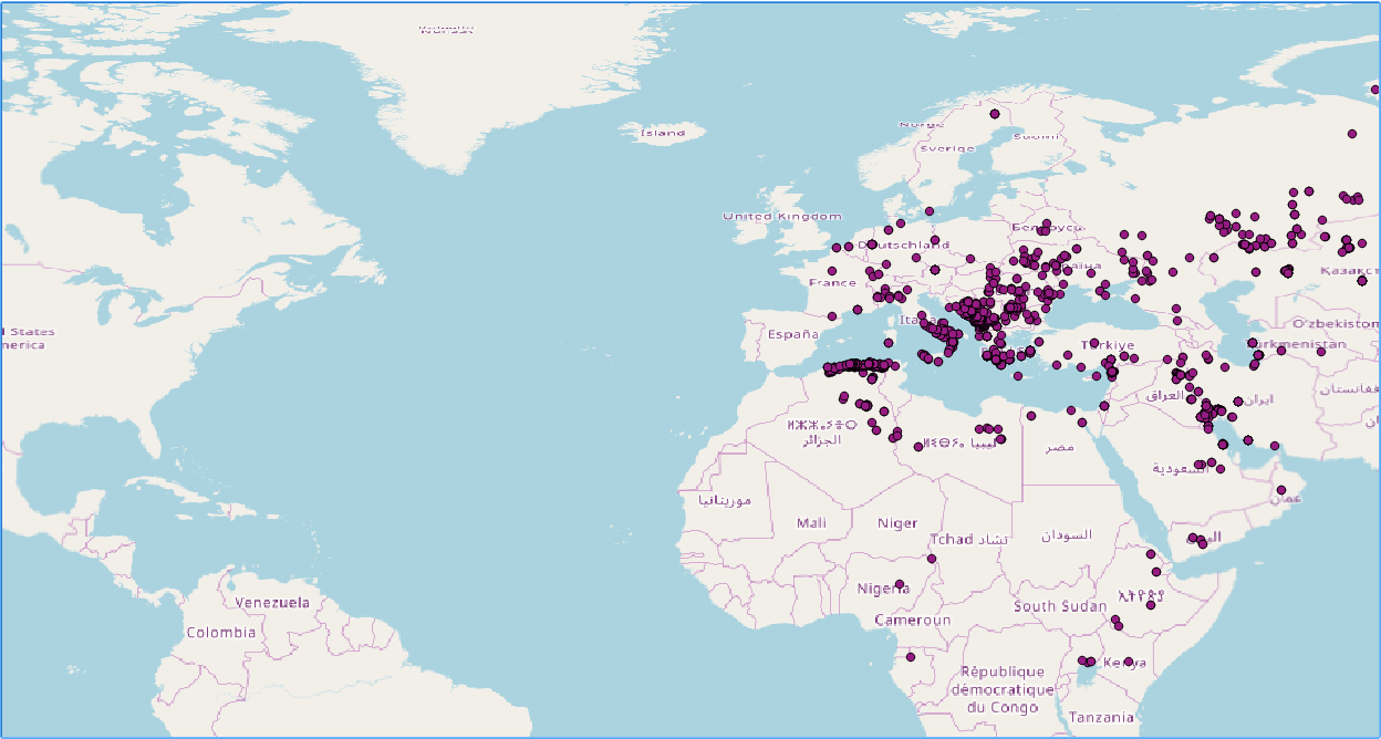
In this recipe, a basic setup for geographical sharding is demonstrated. More sophisticated functions can be implemented easily on the same proposed structure. In addition, for heavy lifting applications purposes, there are some products in the market that could be explored, if considered necessary.
The example shown was based partly on a GitHub implementation found at the following link: https://gist.github.com/sylr/623bab09edd04d53ee4e.
Similar to sharding, working with a large amount of rows within a geospatial table in postgres, will cause a lot of processing time for a single worker. With the release of postgres 9.6, the server is capable of executing queries which can be processed by multiple CPUs for a faster answer. According to the postgres documentation, depending of the table size and the query plan, there might not be a considerable benefit when implementing a parallel query, instead of a serial query.
For this recipe, we need a specific version of postgres. It is not mandatory for you to download and install the postgres version that will be used. The reason is that, some developers might have an already configured postgres database version with data, and having multiple servers running within a computer might cause issues later.
To overcome this problem, we will make use of a docker container. A container could be defined as a lightweight instantiation of a software application that is isolated from other containers and your computer host. Similar to a virtual machine, you could have multiple versions of your software stored inside your host, and start multiple containers whenever necessary.
First, we will download docker from https://docs.docker.com/install/ and install the Community Edition (CE) version. Then, we will pull an already precompiled docker image. Start a Terminal and run the following command:
$ docker pull shongololo/postgis
This docker image has PostgreSQL 10 with Postgis 2.4 and SFCGAL plugin. Now we need to start an instance given the image. An important part corresponds to the -p 5433:5432. These arguments maps every connection and request that is received at port 5433 in your host (local) computer to the 5432 port of your container:
$ docker run --name parallel -p 5433:5432 -v <SHP_PATH>:/data shongololo/postgis
Now, you can connect to your PostgreSQL container:
$ docker exec -it parallel /bin/bash
root@d842288536c9:/# psql -U postgres
psql (10.1)
Type "help" for help.
postgres=#
Where root and d842288536c9 corresponds to your container username and group respectively.
Because we created an isolated instance of your postgres database, we have to recreate to use, database name and schema. These operations are optional. However, we encourage you to follow this to make this recipe consistent with the rest of the book:
root@d842288536c9:/# psql -U postgres
psql (10.1)
Type "help" for help.
postgres=# CREATE USER me WITH PASSWORD 'me';
CREATE ROLE
postgres=# ALTER USER me WITH SUPERUSER;
ALTER ROLE
root@d842288536c9:/# PGPASSWORD=me psql -U me -d postgres
postgres=# CREATE DATABASE "postgis-cookbook";
CREATE DATABASE
postgres=# \c postgis-cookbook
You are now connected to database postgis-cookbook as user me:
postgis-cookbook=# CREATE SCHEMA chp10;
CREATE SCHEMA
postgis-cookbook=# CREATE EXTENSION postgis;
CREATE EXTENSION
root@d842288536c9:/# /usr/lib/postgresql/10/bin/shp2pgsql -s 3734
-W latin1 /data/gis.osm_buildings_a_free_1.shp chp10.buildings |
PGPASSWORD=me psql -U me -h localhost -p 5432 -d postgis-cookbook
The second option is in your host computer. Make sure to correctly set your shapefiles path and host port that maps to the 5432 container port. Also, your host must have postgresql-client installed:
$ shp2pgsql -s 3734 -W latin1 <SHP_PATH>
/gis.osm_buildings_a_free_1.shp chp10.buildings | PGPASSWORD=me
psql -U me -h localhost -p 5433 -d postgis-cookbook
postgis-cookbook=# EXPLAIN ANALYZE SELECT Sum(ST_Area(geom))
FROM chp10.buildings;
We get the following result:
Aggregate (cost=35490.10..35490.11 rows=1 width=8)
(actual time=319.299..319.2 99 rows=1 loops=1)
-> Seq Scan on buildings (cost=0.00..19776.16 rows=571416 width=142)
(actual time=0.017..68.961 rows=571416 loops=1)
Planning time: 0.088 ms
Execution time: 319.358 ms
(4 rows)
Now, if we modify the max_parallel_workers and max_parallel_workers_per_gather parameters, we activate the parallel query capability of PostgreSQL:
Aggregate (cost=35490.10..35490.11 rows=1 width=8)
(actual time=319.299..319.299 rows=1 loops=1)
-> Seq Scan on buildings (cost=0.00..19776.16 rows=571416 width=142)
(actual time=0.017..68.961 rows=571416 loops=1)
Planning time: 0.088 ms
Execution time: 319.358 ms
(4 rows)
This command prints in Terminal:
Finalize Aggregate (cost=21974.61..21974.62 rows=1 width=8)
(actual time=232.081..232.081 rows=1 loops=1)
-> Gather (cost=21974.30..21974.61 rows=3 width=8)
(actual time=232.074..232.078 rows=4 loops=1)
Workers Planned: 3
Workers Launched: 3
-> Partial Aggregate (cost=20974.30..20974.31 rows=1 width=8)
(actual time=151.785..151.785 rows=1 loops=4)
-> Parallel Seq Scan on buildings
(cost=0.00..15905.28 rows=184328 width=142)
(actual time=0.017..58.480 rows=142854 loops=4)
Planning time: 0.086 ms
Execution time: 239.393 ms
(8 rows)
postgis-cookbook=# EXPLAIN ANALYZE SELECT * FROM chp10.buildings
WHERE ST_Area(geom) > 10000;
We get the following result:
Seq Scan on buildings (cost=0.00..35490.10 rows=190472 width=190)
(actual time=270.904..270.904 rows=0 loops=1)
Filter: (st_area(geom) > '10000'::double precision)
Rows Removed by Filter: 571416
Planning time: 0.279 ms
Execution time: 270.937 ms
(5 rows)
This query is not executed in parallel. This happens because ST_Area function is defined with a COST value of 10. A COST for PostgreSQL is a positive number giving the estimated execution cost for a function. If we increase this value to 100, we can get a parallel plan:
postgis-cookbook=# ALTER FUNCTION ST_Area(geometry) COST 100;
postgis-cookbook=# EXPLAIN ANALYZE SELECT * FROM chp10.buildings
WHERE ST_Area(geom) > 10000;
Now we have a parallel plan and 3 workers are executing the query:
Gather (cost=1000.00..82495.23 rows=190472 width=190)
(actual time=189.748..189.748 rows=0 loops=1)
Workers Planned: 3
Workers Launched: 3
-> Parallel Seq Scan on buildings
(cost=0.00..62448.03 rows=61443 width=190)
(actual time=130.117..130.117 rows=0 loops=4)
Filter: (st_area(geom) > '10000'::double precision)
Rows Removed by Filter: 142854
Planning time: 0.165 ms
Execution time: 190.300 ms
(8 rows)
postgis-cookbook=# DROP TABLE IF EXISTS chp10.pts_10;
postgis-cookbook=# CREATE TABLE chp10.pts_10 AS
SELECT (ST_Dump(ST_GeneratePoints(geom, 10))).geom
::Geometry(point, 3734) AS geom,
gid, osm_id, code, fclass, name, type FROM chp10.buildings;
postgis-cookbook=# CREATE INDEX pts_10_gix
ON chp10.pts_10 USING GIST (geom);
Now, we can run a table join between two tables, which does not give us a parallel plan:
Nested Loop (cost=0.41..89034428.58 rows=15293156466 width=269)
-> Seq Scan on buildings (cost=0.00..19776.16 rows=571416 width=190)
-> Index Scan using pts_10_gix on pts_10
(cost=0.41..153.88 rows=190 width=79)
Index Cond: (buildings.geom && geom)
Filter: _st_intersects(buildings.geom, geom)
For this case, we need to modify the parameter parallel_tuple_cost which sets the planner's estimate of the cost of transferring one tuple from a parallel worker process to another process. Setting the value to 0.001 gives us a parallel plan:
Nested Loop (cost=0.41..89034428.58 rows=15293156466 width=269)
-> Seq Scan on buildings (cost=0.00..19776.16 rows=571416 width=190)
-> Index Scan using pts_10_gix on pts_10
(cost=0.41..153.88 rows=190 width=79)
Index Cond: (buildings.geom && geom)
Filter: _st_intersects(buildings.geom, geom)
As demonstrated in this recipe, parallelizing queries in PostgreSQL allows the optimization of operations that involve a large dataset. The database engine is already capable of implementing parallelism, but defining the proper configuration is crucial in order to take advantage of the functionality.
In this recipe, we used the max_parallel_workers and the parallel_tuple_cost to configure the desired amount a parallelism. We could evaluate the performance with the ANALYZE function.
In this chapter, we will cover the following topics:
At a minimum, desktop GIS programs allow you to visualize data from a PostGIS database. This relationship gets more interesting with the ability to edit and manipulate data outside of the database and in a dynamic play environment.
Make a change, see a change! For this reason, visualizing the data stored in PostGIS is often critical for effective spatial database management—or at least as a now-and-again sanity check. This chapter will demonstrate both dynamic and static relationships between your database and desktop clients.
Regardless of your experience level or role in the geospatial community, you should find at least one of the four GIS programs serviceable as a potential intermediate staging environment between your PostGIS database and end product.
In this chapter, we will connect to PostGIS using the following desktop GIS programs: QGIS, OpenJUMP GIS, gvSIG, and uDig.
Once connected to PostGIS, extra emphasis will be placed on some of the more sophisticated functionalities offered by QGIS and OpenJUMP GIS using the Database Manager (DB Manager) plugin and data store queries, respectively.
In this recipe, we will establish a connection to our PostGIS database in order to add a table as a layer in QGIS (formerly known as Quantum GIS). Viewing tables as layers is great for creating maps or simply working on a copy of the database outside the database.
Please navigate to the following site to install the latest version LTR of QGIS (2.18 – Las Palmas at the time of writing):
On this page, click on Download Now and you will be able to choose a suitable operating system and the relevant settings. QGIS is available for Android, Linux, macOS X, and Windows. You might also be inclined to click on Discover QGIS to get an overview of basic information about the program along with features, screenshots, and case studies.
To begin, create the schema for this chapter as chp11; then, download data from the U.S. Census Bureau's FTP site:
http://ftp2.census.gov/geo/tiger/TIGER2012/EDGES/tl_2012_39035_edges.zip
The shapefile is All Lines for Cuyahoga county in Ohio, which consist of roads and streams among other line features.
Use the following command to generate the SQL to load the shapefile in a table of the chp11 schema:
shp2pgsql -s 4269 -W LATIN1 -g the_geom -I tl_2012_39035_edges.shp chp11.tl_2012_39035_edges > tl_2012_39035_edges.sql
Now it's time to give the data we downloaded a look using QGIS. We must first create a connection to the database in order to access the table. Get connected and add the table as a layer by following the ensuing steps:
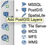
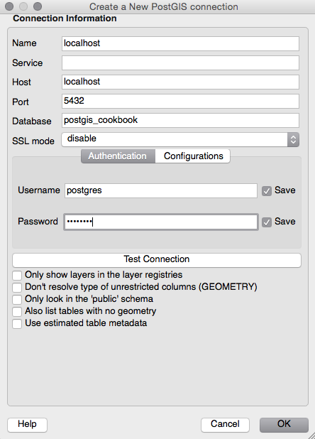
Make sure the name of your PostGIS connection appears in the drop-down menu and then click on the Connect button. If you choose not to store your username and password, you will be asked to submit this information every time you try to access the database.
Once connected, all schemas within the database will be shown and the tables will be made visible by expanding the target schema.
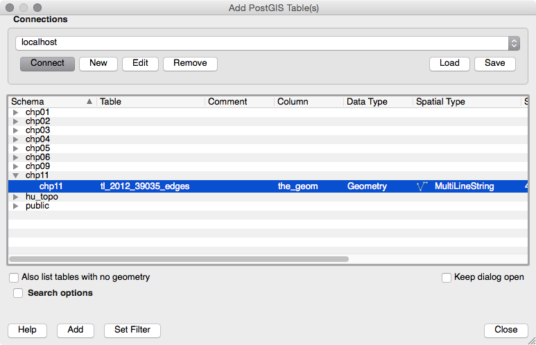
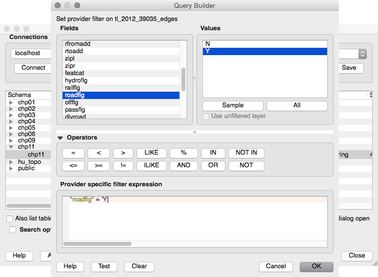
The same holds true the other way around. Changes to the table in the database will have no effect on the layer in QGIS.
If needed, you can save the temporary layer in a variety of formats, such as DXF, GeoJSON, KML, or SHP. Simply right-click on the layer name in the Layers panel and click on Save As. This will then create a file, which you can recall at a later time or share with others.
The following screenshot shows the Cuyahoga county road network:
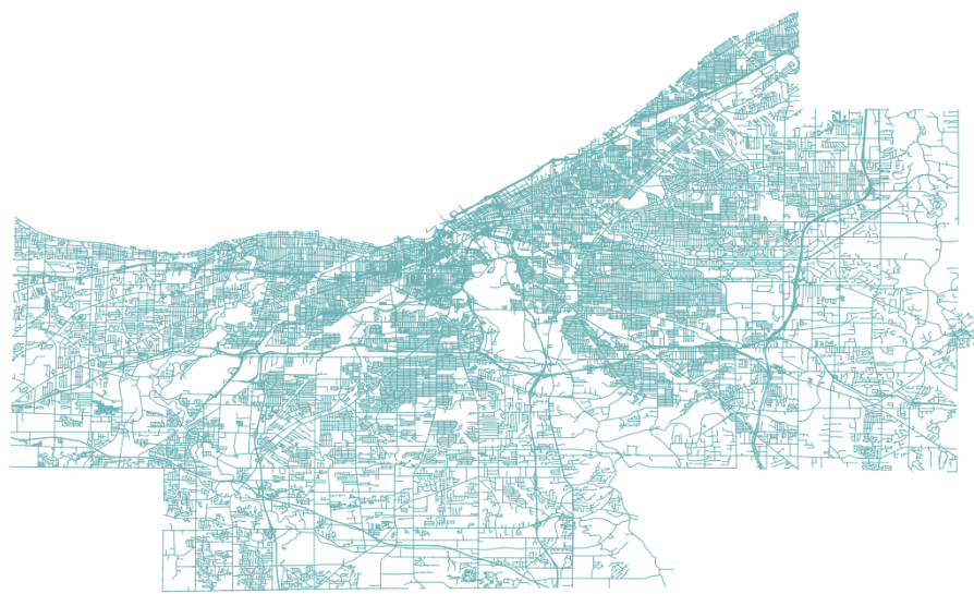
You may also use the QGIS Browser Panel to navigate through the now connected PostGIS database and list the schemas and tables. This panel allows you to double-click to add spatial layers to the current project, providing a better user experience not only of connected databases, but on any directory of your machine:
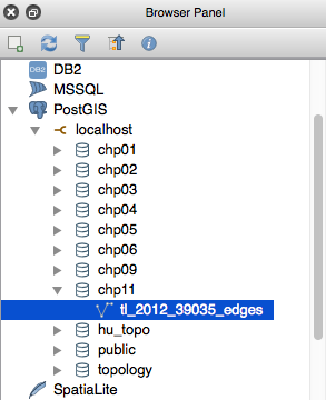
You have added a PostGIS layer into QGIS using the built-in Add PostGIS Table GUI. This was achieved by creating a new connection and entering your database parameters.
Any number of database connections can be set up simultaneously. If working with multiple databases is more common for your workflows, saving all of the connections into one XML file (see the tip in the preceding section) would save time and energy when returning to these projects in QGIS.
Database Manager (DB Manager) allows for a more sophisticated relationship with PostGIS by allowing users to interact with the database in a variety of ways. The plugin mimics some of the core functionality of pgAdmin with the added benefit of data visualization.
In this recipe, we will use DB Manager to create, modify, and delete items within the database and then tinker with the SQL window. By the end of this section, you will be able to do the following:
QGIS needs to be installed for this recipe. Please refer to the first recipe in this chapter for information on where to download the installer.
Let's make sure the plugin is enabled and connected to the database.
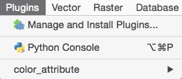
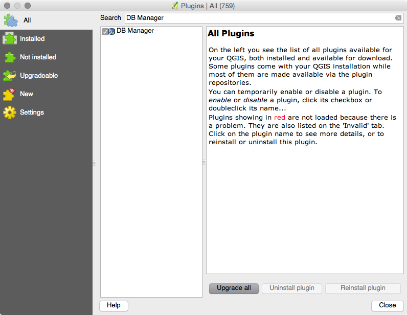

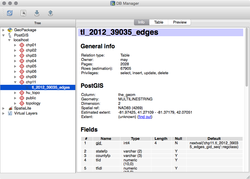
A PostGIS connection is not in place if you are unable to expand the PostGIS menu. If you need to establish a connection, refer to steps 1 to 4 in the Adding PostGIS layers – QGIS recipe. The connection must be established before using DB Manager.
Navigate to the DB Manager menu and carry out the following steps:
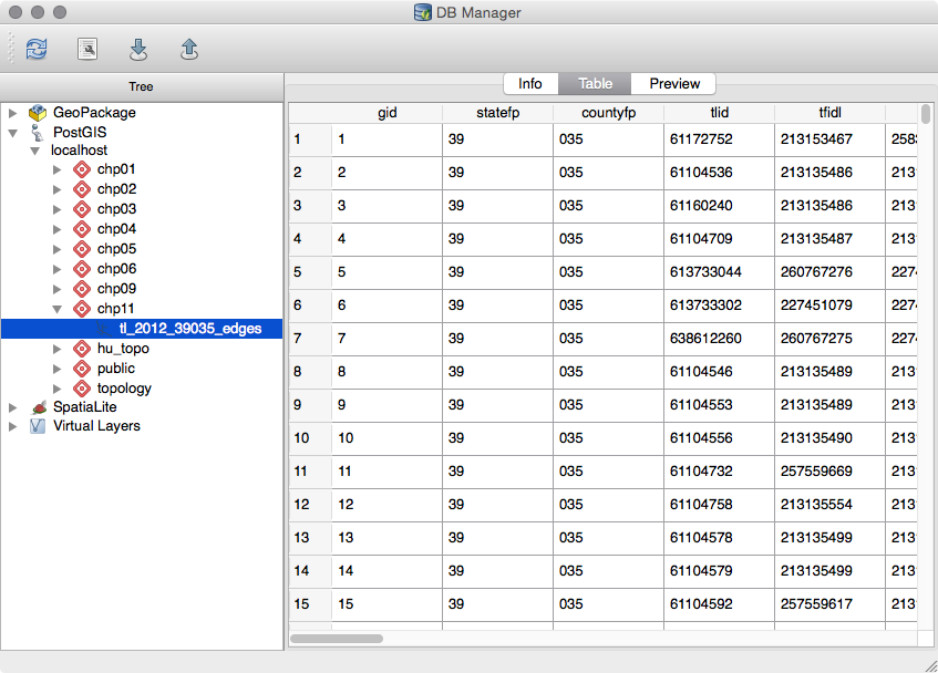
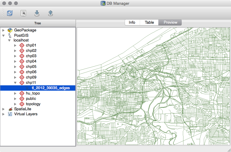
To create, modify, and delete database schemas and tables, follow the ensuing steps:

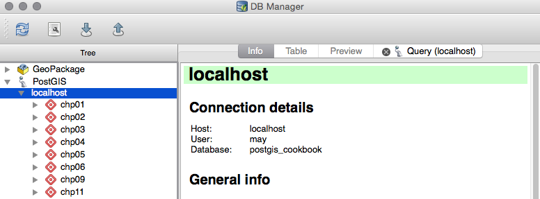
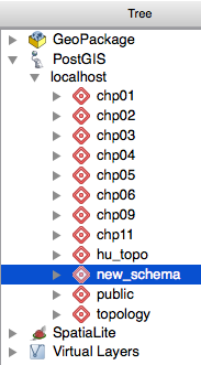
Now let's continue to work with our chp11 schema containing the tl_2012_39035_edges table. Let's modify the table name to something more generic. How about lines? You can change the table name by clicking on the table in the Tree window. As soon as the text is highlighted and the cursor flashes, you can delete the existing name and enter the new name, lines.
Right now, our lines table's data is using degrees as the unit of measurement for its current projection (EPSG: 4269). Let's add a new geometry column using EPSG: 3734, which is a State Plane Coordinate system that measures projections in feet. To run SQL queries, follow the ensuing steps:
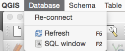
SELECT AddGeometryColumn('chp11', 'lines','geom_sp',3734,
'MULTILINESTRING', 2);
UPDATE "chp11".lines
SET geom_sp = ST_Transform(the_geom,3734);
The query creates a new geometry column named geom_sp and then updates the geometry information by transforming the original geometry (geom) from EPSG 4269 to 3734, as shown in the following screenshot:
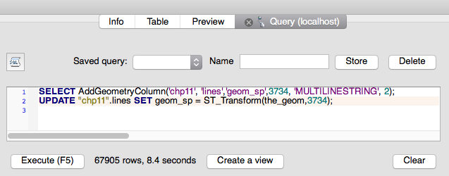
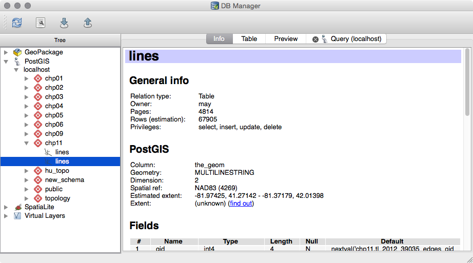
The preceding screenshot shows the original geometry. The following screenshot shows the created geometry:
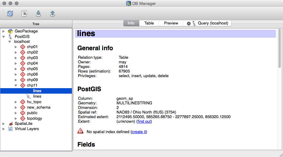
SELECT gid, ST_Buffer(geom_sp, 10) AS geom, fullname, roadflg
FROM "chp11".lines WHERE roadflg = 'Y'
Check the Load as new layer checkbox and then select gid as the unique ID and geom as the geometry. Create a name for the layer and then click on Load Now!, and what you'll see is shown in the following screenshot:
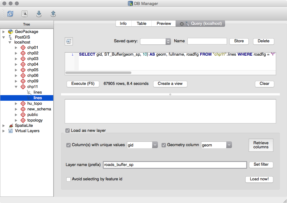
The query adds the result in QGIS as a temporary layer.
CREATE TABLE "chp11".roads_buffer_sp AS SELECT gid,
ST_Buffer(geom_sp, 10) AS geom, fullname, roadflg
FROM "chp11".lines WHERE roadflg = 'Y'
The following screenshot shows the Cuyahoga county road network:
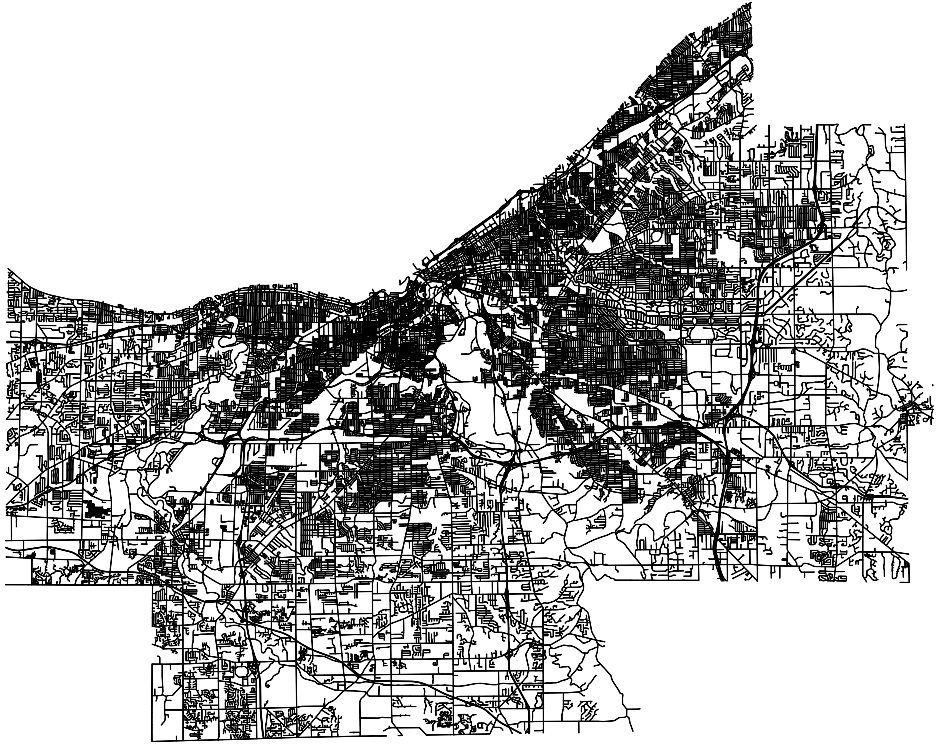
Connecting to a PostGIS database (see the Adding PostGIS layers – QGIS recipe in this chapter) allows you to utilize the DB Manager plugin. Once DB Manager was enabled, we were able to toggle between the Info, Table, and Preview tabs to efficiently view metadata, tabular data, and data visualization.
Next, we made changes to the database through the query window, running on the table lines of schema chp11 in order to transform the projection. Note the autocomplete feature in the SQL Window, which makes writing queries a breeze.
Changes to the database were made visible in DB Manager by refreshing the database connection.
In this section, we will connect to PostGIS with OpenJUMP GIS (OpenJUMP) in order to add spatial tables as layers. Next, we will edit the temporary layer and update it in a new table in the database.
The JUMP in OpenJUMP stands for Java Unified Mapping Platform. To learn more about the program, or if you need to install the latest version, go to:
Click on the Download latest version link (http://sourceforge.net/projects/jump-pilot/files/OpenJUMP/1.12/) on the page to view the list of installers. Select the version that suits your operating system (.exe for Windows and .jar for Linux and mac OS). Detailed directions for installing OpenJUMP along with other documentation and information can be found on the OpenJUMP Wiki page at the following link:
We will be reusing and building upon data used in the Adding PostGIS layers – QGIS recipe. If you skipped over this recipe, you will want to do the following:
ftp://ftp2.census.gov/geo/tiger/TIGER2012/EDGES/tl_2012_39035_edges.zip
The shapefile is All Lines for Cuyahoga county in Ohio, which consist of roads and streams, among other line features.
The data source layer can be added by performing the following steps:
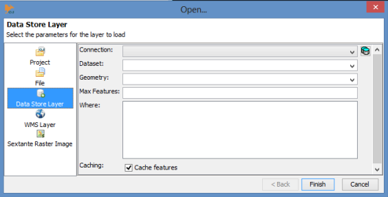
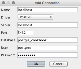
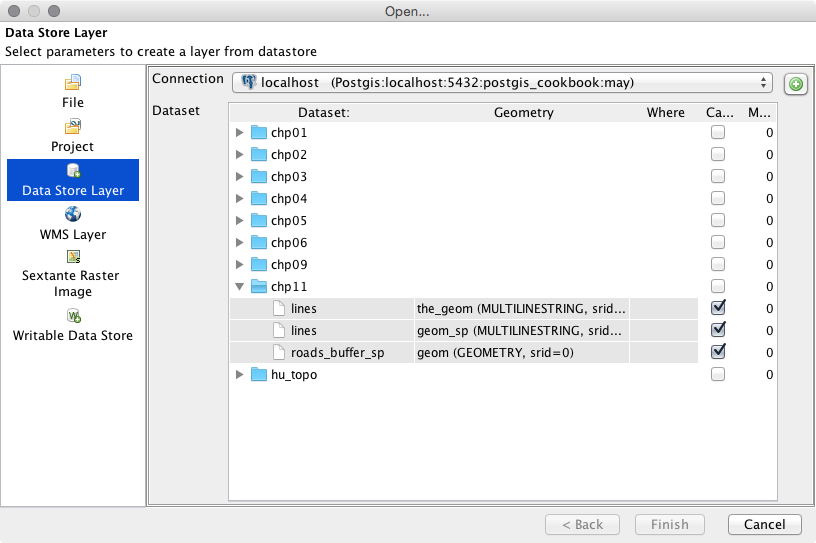
If multiple geometry columns exist, you may choose the one you want to use. Add the data's state plane coordinator geometry (geom_sp), as shown in the Using the Database Manager plugin – QGIS recipe.
Simple SQL WHERE clause statements can be used if only a subset of a table is needed.
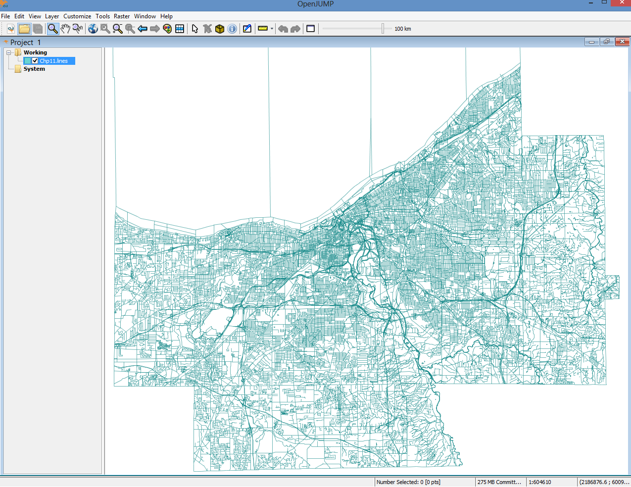

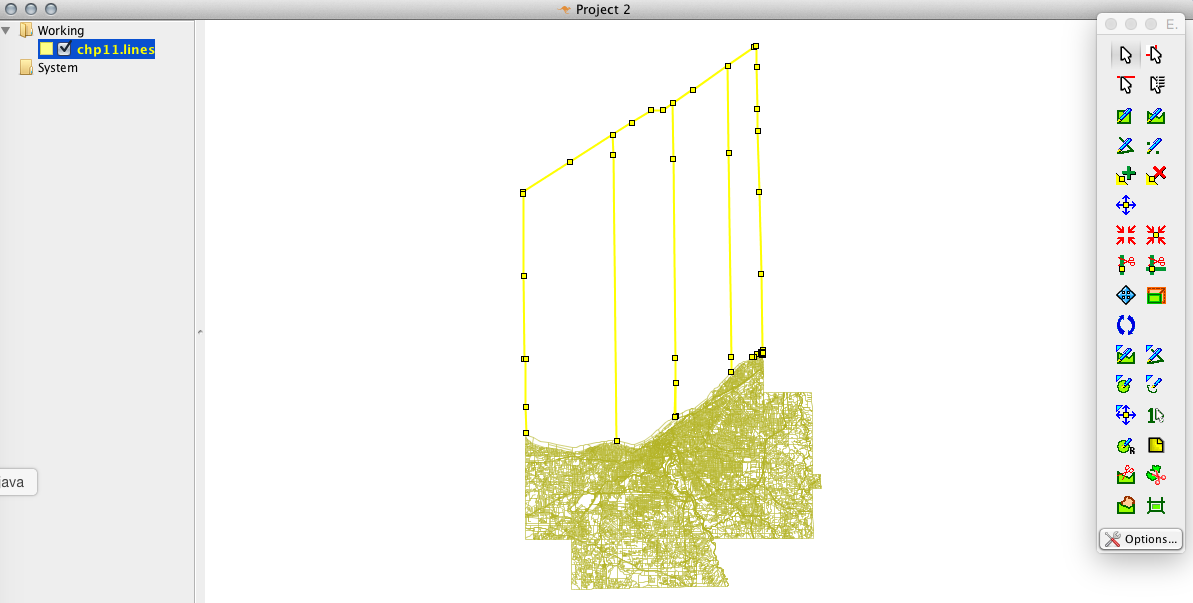
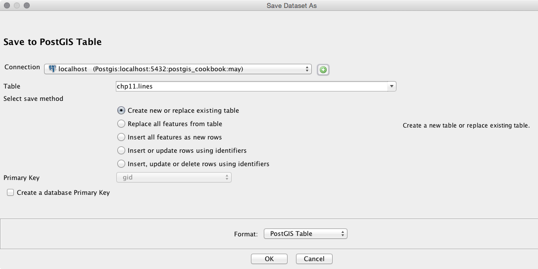
We added a PostGIS layer in OpenJUMP using the Open Data Store Layer menu. This was achieved after creating a new connection and entering our database parameters.
In the example, census data was added which included the boundary of Cuyahoga county. Part of the boundary advances into Lake Erie to the International Boundary with Canada. While technically correct, the water boundary is typically not used for practical mapping purposes. In this case, it's easy to visualize which data needs to be removed.
OpenJUMP allows us to easily see and delete records that should be deleted from the table. The selected lines were deleted, and the table was saved to the database.
Executing ad hoc queries in OpenJUMP is simple and offers a couple of unique features. Queries can be run on specific data selections, allowing for the manual control of the queried area without considering the attribution. Similarly, temporary fences (areas) can be drawn on the fly and the geometry of the surface can be used in queries. In this recipe, we will explore each of those cases.
Refer to the preceding recipe if you need to install OpenJUMP or require assistance connecting to a database.
Carry out the following steps to run the data store query:
SELECT gid, ST_BUFFER("chp11".lines.geom_sp, 75)
AS the_geom, fullname
FROM "chp11".lines WHERE fullname <> '' AND hydroflg = 'Y'
The preceding query is shown in the following screenshot:
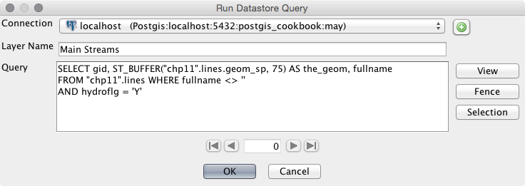
The preceding query selects the lines on the map that represent hydrology units such as "hydroflg" = 'Y' and streams. The selected stream lines (which use the State Plane geometry) are buffered by 75 feet, which should yield a result like that shown in the following screenshot:
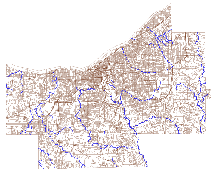
SELECT AddGeometryColumn('chp11', 'lines','geom_sp',3734,
'MULTILINESTRING', 2);
UPDATE "chp11".lines SET geom_sp = ST_Transform(geom,3734);

You should now have a fence junction between the selected polygons. You should see something similar to the following screenshot:
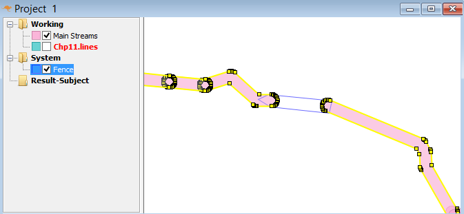
Run ST_UNION on the selection and fence together so that the gap is filled. We do this with the following query:
SELECT ST_UNION(geom1, geom2) AS geom
Use the Selection and Fence buttons in place of geom1 and geom2 so that your query looks as shown in the following screenshot:
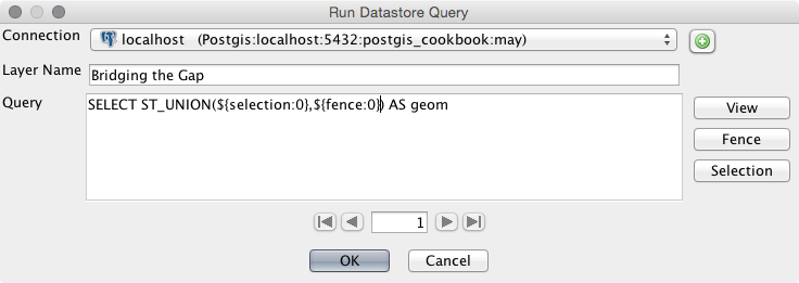

We added a buffered subset of a PostGIS layer in OpenJUMP using the Run Datastore Query menu. We took lines from a database table and converted them to polygons to view them in OpenJUMP.
We then manually selected an area of interest that had two representative stream polygons disjointed from one another, the idea being that the streams would be, or are, connected in a natural state.
The Fence tool was used to draw a freehand polygon between the streams. A union query was then performed to combine the two stream polygons and the fences. Fences allow us to create temporary tables for use in spatial queries executed against a database table.
gvSIG is a GIS package developed for the Generalitat Valenciana (gv) in Spain. SIG is the Spanish equivalent of GIS. Intended for use all over the world, gvSIG is available in more than a dozen languages.
Installers, documentation, and more details for gvSIG can be found at the following website:
To download gvSIG, click on the latest version (gvSIG 2.0 at the time of writing). The all-included version is recommended on the gvSIG site. Be careful while selecting the .exe or .bin versions; otherwise, you may download the program in a language that you don't understand.
The GeoDB layer can be added by following the ensuing steps:
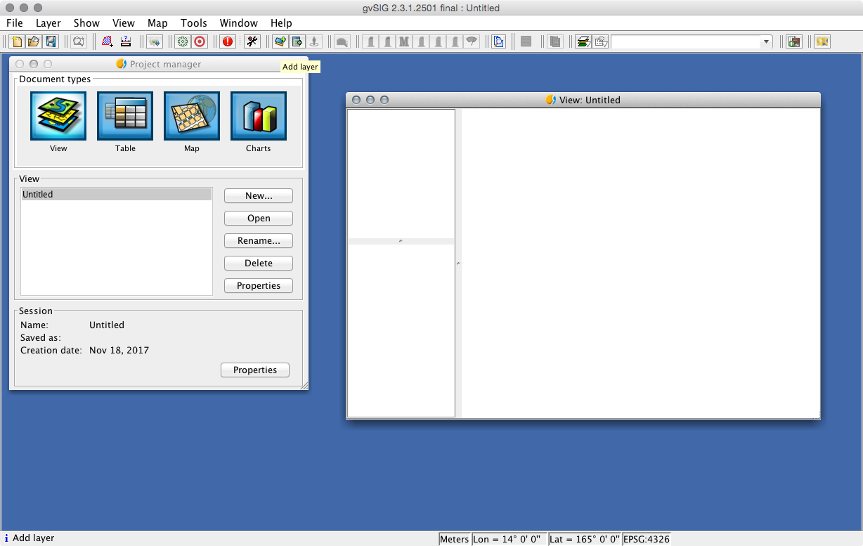
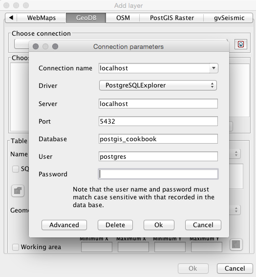
You can see these steps performed in the following screenshot:
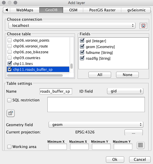
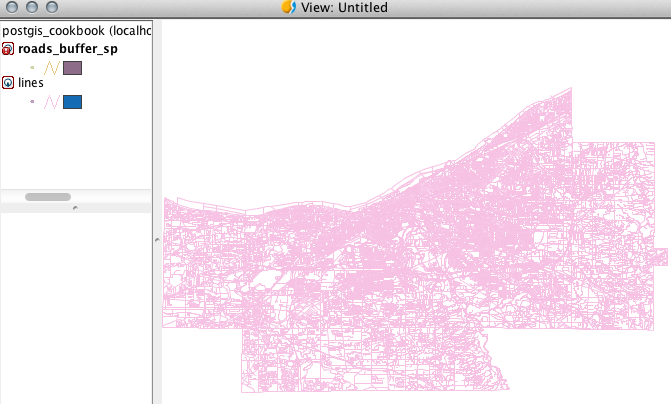
PostGIS layers were added to gvSIG using the Add Layer menu. The GeoDB tab allowed us to set the PostGIS connection. After choosing a table, many options are afforded with gvSIG. The layer name can be aliased to something more meaningful and unnecessary columns can be omitted from the table.
A hallmark of the User-friendly Desktop Internet GIS (uDig) program built with Eclipse is that it can be used as a standalone application or a plugin for existing applications. Details on the uDig project as well as installers can be found at the following website:
Click on Downloads at the preceding website to view the list of versions and installers. At the time of writing, 2.0.0.RC1 is the latest stable version. uDig is supported by Windows, macOS X, and Linux.
In this recipe, we will quickly connect to a PostGIS database and then add a layer to uDig.
Carry out the following steps:
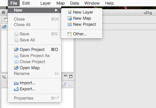
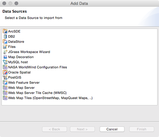
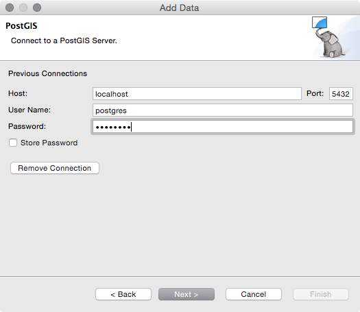
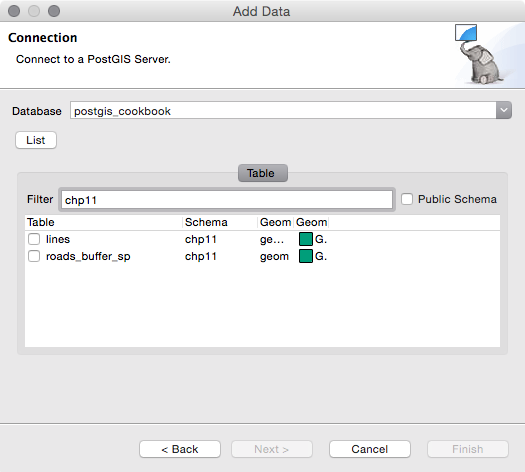
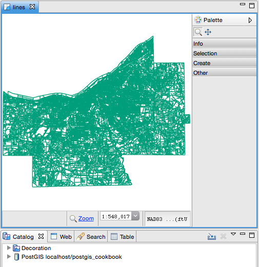
The New Layer menu in uDig generates a hefty list of possible sources that can be added. PostGIS was set as the database and your database parameters were entered. uDig was then connected to the database. Clicking on List displays the total number of tables available in the connected database. Any number of tables can be added at once.
In this chapter, we will cover the following recipes:
This chapter is dedicated to an emerging issue in the design and implementation of location-based information systems: LBISs. The increasing use of smartphones in all kinds of applications, and their ability to acquire and report users' locations, has been adopted as a core functionality of many service providers. Enabling access to users' accurate locations throughout the day, which gives context to their requests and allows companies to better know their client and provide any relevant personalized services; however, this information can contain much more about the user than just the context of the service they want to access, such as their weekly routine, frequently visited places, groups of people gathered, and so on. These patterns can be obtained from the phone, and then analyzed and used to categorize or profile customers; this information in the wrong hands, however, could be used against individuals.
Even though there is very little [1] to no regulation on how to handle location information in a way that guarantees privacy for users, it is very important that the proper policies and implementation are included at the design stage.
Fortunately, among geoprivacy researchers, there exists a wide variety of mechanisms that can be used to help mitigate the issue of privacy in LBISs.
This chapter is somewhat different from the others because, in order to understand the background of each location privacy technique, we considered important to include the theoretical bases that support these recipes that to the best of our knowledge are only available through academic publications and not yet presented as a hands-on experience.
Location privacy can be defined by Duckham and Kulik in [2] as follows: A special type of information privacy which concerns the claim of individuals to determine for themselves when, how, and to what extent location information about them is communicated to others. Based on this definition, users should have power over their location information; however, it is well known that this is not the reality in many cases. Often, a service provider requires full access to a user's location in order for the service to become available.
In addition, because there is no restriction on the quality of location information that service providers can record, it's common for the exact GPS coordinates to be acquired, even when it is not relevant to the service itself.
The main goal of LPPMs should be to allow users to hide or reduce the quality of this location information in such a way that users will still have an adequate service functionalities, and that the service provider can still benefit from insights product of spatial analysis .
In order to provide geoprivacy, it is important to understand the components location information, these are: identity, location, and time. If an adversary is able to link those three aspects, location privacy is compromised. These components form an instance of location information; a sequence of such instances that gives historical location information, allowing others to establish behavior patterns and then making it possible for them to identify the user's home, work, and routine. Most LPPMs attack at least one of these components in order to protect privacy.
Suppose an attacker gains access to a user's identity and the time, but has no clear knowledge of what places the user has visited. As the location component has been obfuscated, the attacker would be able to infer very little, as the context is highly-altered and the data has lost its potential usability. (This specific scenario corresponds to location privacy.)
Another popular solution has been the implementation of identity privacy or anonymity, where users' traveled pathways can be accessed, but they provide no information on the identity of the subjects, or even if they are different users; however, this information alone could be enough to infer the identity of a person by matching records on a phonebook, as in the experiments conducted by [3].
Finally, when a user's location and identity are specified, but the time component is missing, the resulting information lacks context, and so pathways may not be reconstructed accurately; however, implementing a model in which this occurs is unlikely, as requests and LBS responses happen at a specific time and delaying queries can cause them to lose their relevance.
Privacy in location-based services is often viewed as reaching a desirable trade-off between performance and a user's privacy; the more privacy provided, the less likely it is that the service can function as it would under a no-privacy scheme, or without suffering alterations in their architecture or application layer. As LBS offers a great variety of ever-changing features that keep up with users' needs while making use of the latest available technologies and adjusting to social behavior, they provide a similar scenario to LPPMs that aims to cover these services.
In the case of proactive location-based services (PLBS), where users are constantly reporting their location [4], the purpose of LPPMs is to alter the route as much as possible, while still providing a minimum level of accuracy that will allow the LBS to provide relevant information. This can be challenging because many PLBS, like traffic guidance apps, require the exact location of the user. So, unless the original data can be recovered or used in the altered format, it would be very complicated for these applications to implement an LPPM. Other services, like geomarketing or FriendFinder, may tolerate a larger alteration of the data, even if the change cannot be undone.
On the other hand, mechanisms intended for reactive location-based services (RLBS) often do not require critical accuracy, and therefore it is tolerable to alter the subject's position in order to provide location privacy.
Some LPPMs require special features alongside the usual client-server architecture, such as special database structures, extra data processing layers, third-party services, proxies, special electronics, a peer-to-peer approach between the LBS users' community, and so on.
Based on this, a proposed way to classify LPPMs is based on the application to PLBS and RLBS. Some of the techniques are general enough that they can be used in both worlds, but each has different implications:

In this chapter, two examples of LPPM implementations will be shown: noise-based location obfuscation, and private-information retrieval. Each of these imply changes to the design of the LBIS and the geographical database.
Some of the mechanisms designed for location privacy protection are based on location obfuscation, which is explained in [5] as the means of deliberately degrading the quality of information about an individual's location in order to protect that individual's location privacy.
This is perhaps the simplest way to implement location privacy protection in LBISs because it has barely any impact on the server-side of the application, and is usually easy to implement on the client-side. Another way to implement it would be on the server-side, running periodically over the new data, or as a function applied to every new entry.
The main goal of these techniques is to add random noise to the original location obtained by the cellphone or any other location-aware device, so as to reduce the accuracy of the data. In this case, the user can usually define the maximum and/or minimum amount of noise that they want to add. The higher the noise added, the lower the quality of the service; so it is very important to reasonably set this parameter. For example, if a real-time tracking application receives data altered by 1 km, the information provided to the user may not be relevant to the real location.
Each noise-based location obfuscation technique presents a different way to generate noise:
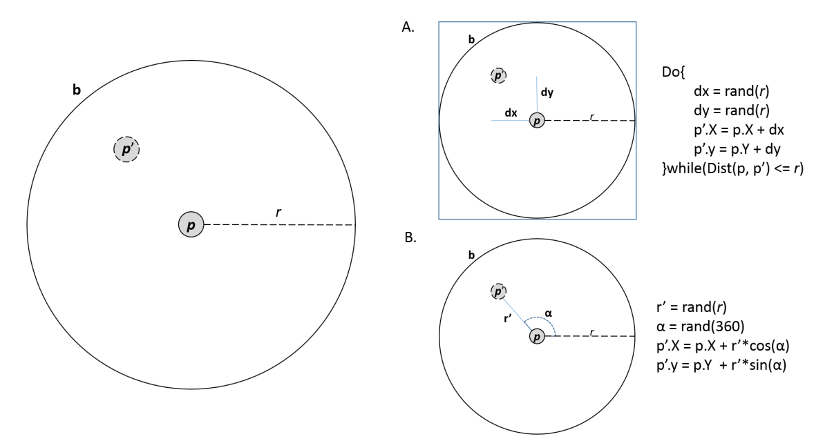
When the noise is generated with polar coordinates, it is more uniformly distributed over a projection of the circular area because both angle and distance follow that distribution. In the case of Cartesian-based noise, points appear to be generated uniformly among the area as a whole, resulting in a lower density of points near the center. The following figure shows the differences in both circular and rectangular projections of 500 random points. In this book, we will work with polar-based random generation:
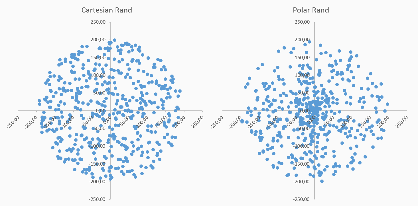
The following figure illustrates the way the N-RAND [6], θ-RAND [7], and Pinwheel [8] techniques work:
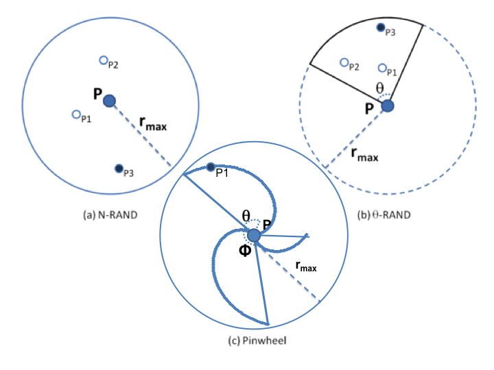
N-RAND generates N points in a given area, and selects the point furthest away from the center. Θ-RAND does the same, but in a specific sector of the circular area. There can be more than just one area to select from. Finally, the Pinwheel mechanism differs from N-RAND and θ-RAND because it does not generate random distances for the points, and instead defines a specific one for each angle in the circumference, making the selection of the radius a more deterministic process when generating random points. In this case, the only random variable in the generation process is the angle α. The formula to calculate the radius for a given angle, α, is presented in (1), as follows:

Where φ is a preset parameter defined by the user, it determines the amplitude of the wings of geometry, which resembles a pinwheel.
The lower the value of φ, the more wings the pinwheel will have, but those wings will also be thinner; on the other hand, the higher the value, the fewer the number of wider wings:
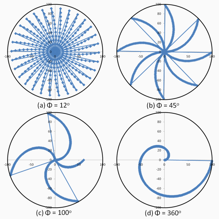
Once the locations have been altered, it is very unlikely that you will be able to recover the original information; however, filtering noise techniques are available in the literature that reduce the impact of alterations and allow a better estimation of the location data. One of these mechanisms for noise-filtering is based on an exponential moving average (EMA) called Tis-Bad [9].
There is still an open discussion on how much degradation of the location information is sufficient to provide location privacy to users, and moreover, if the resulting obfuscated information remains useful when accessing a LBS. After all, obtaining relevant responses while performing geospatial analysis is one of the main issues regarding LBS and the study of geo-referenced data.
In this recipe, we will create PLPGSQL functions that implement three noise-based obfuscation mechanisms: Rand, N-Rand, and Pinwheel. Then we will create a trigger function for a table in order to alter all newly inserted points. For this chapter, we will reuse the rk_track_points dataset used in Chapter 3, Working with Vector Data – The Basics.
In this recipe, we will use the ST_Project function to add noise to a single point. Then, we will compare the original data with obfuscated data in QGIS. Finally, we will show the impact of noise filtering on the obfuscated data.
In the recipe, we will use some of the same steps as in Chapter 3, Working with Vector Data – The Basics, but for a new schema.
First, be sure of the format of the .gpx files that you need to import to PostGIS. Open one of them and check the file structure—each file must be in the XML format, composed of one <trk> element, which contains just one <trkseg> element, which contains multiple <trkpt> elements (the points stored from the runner's GPS device).
Carry out the following steps to create the functions:
postgis_cookbook=# create schema chp12;
The ST_Project function will move the point to a given distance and angle from its original location. In order to simplify the expression, we will use polar noise generation. Execute the following SQL command:
postgis_cookbook=# CREATE OR REPLACE
FUNCTION chp12.rand(radius numeric, the_geom geometry)
returns geometry as $$ BEGIN return st_Project(the_geom, random()*radius,
radians(random()*360)); END; $$ LANGUAGE plpgsql;
postgis_cookbook=# CREATE OR REPLACE FUNCTION chp12.nrand(n integer,
radius numeric, the_geom geometry)
returns geometry as $$ DECLARE tempdist numeric; maxdist numeric; BEGIN tempdist := 0; maxdist := 0; FOR i IN 1..n LOOP tempdist := random()*radius; IF maxdist < tempdist THEN maxdist := tempdist; END IF; END LOOP; return st_Project(the_geom,maxdist, radians(random()*360)); END; $$ LANGUAGE plpgsql;
postgis_cookbook=# CREATE OR REPLACE FUNCTION chp12.pinwheel
(theta numeric, radius numeric, the_geom geometry)
returns geometry as $$ DECLARE angle numeric; BEGIN angle = random()*360; return st_Project(the_geom,mod(
CAST(angle as integer), theta)/theta*radius, radians(angle)); END; $$ LANGUAGE plpgsql;
postgis_cookbook=# CREATE TABLE chp12.rk_track_points
(
fid serial NOT NULL,
the_geom geometry(Point,4326),
ele double precision,
"time" timestamp with time zone,
CONSTRAINT activities_pk PRIMARY KEY (fid)
);
This function will return a new geometry:
CREATE OR REPLACE FUNCTION __trigger_rk_track_points_before_insert(
) RETURNS trigger AS $__$
DECLARE
maxdist integer;
n integer;
BEGIN
maxdist = 500;
n = 4;
NEW.the_geom = chp12.nrand(n, maxdist, NEW.the_geom);
RETURN NEW;
END;
$__$ LANGUAGE plpgsql;
CREATE TRIGGER rk_track_points_before_insert
BEFORE INSERT ON chp12.rk_track_points FOR EACH ROW
EXECUTE PROCEDURE __trigger_rk_track_points_before_insert();
The following is the Linux version (name it working/chp03/import_gpx.sh):
#!/bin/bash
for f in `find runkeeper_gpx -name \*.gpx -printf "%f\n"`
do
echo "Importing gpx file $f to chp12.rk_track_points
PostGIS table..." #, ${f%.*}"
ogr2ogr -append -update -f PostgreSQL
PG:"dbname='postgis_cookbook' user='me' password='mypassword'"
runkeeper_gpx/$f -nln chp12.rk_track_points
-sql "SELECT ele, time FROM track_points"
done
The following is the Windows version (name it working/chp03/import_gpx.bat):
@echo off
for %%I in (runkeeper_gpx\*.gpx*) do (
echo Importing gpx file %%~nxI to chp12.rk_track_points
PostGIS table...
ogr2ogr -append -update -f PostgreSQL
PG:"dbname='postgis_cookbook' user='me' password='mypassword'"
runkeeper_gpx/%%~nxI -nln chp12.rk_track_points
-sql "SELECT ele, time FROM track_points"
)
$ chmod 775 import_gpx.sh
$ ./import_gpx.sh
Importing gpx file 2012-02-26-0930.gpx to chp12.rk_track_points
PostGIS table...
Importing gpx file 2012-02-29-1235.gpx to chp12.rk_track_points
PostGIS table...
...
Importing gpx file 2011-04-15-1906.gpx to chp12.rk_track_points
PostGIS table...
In Windows, double-click on the .bat file, or run it from the command prompt using the following command:
> import_gpx.bat
select ST_ASTEXT(rk.the_geom), ST_ASTEXT(rk2.the_geom)
from chp03.rk_track_points as rk, chp12.rk_track_points as rk2
where rk.fid = rk2.fid
limit 10;
The results of the query are as follows:
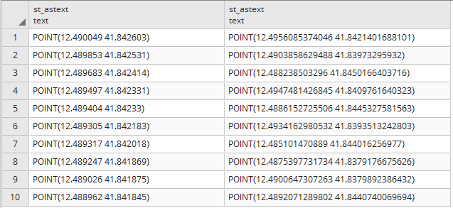
CREATE TABLE chp12.rk_points_rand_500 AS (
SELECT chp12.rand(500, the_geom)
FROM chp12.rk_track_points
);
CREATE TABLE chp12.rk_points_rand_1000 AS (
SELECT chp12.rand(1000, the_geom)
FROM chp12.rk_track_points
);
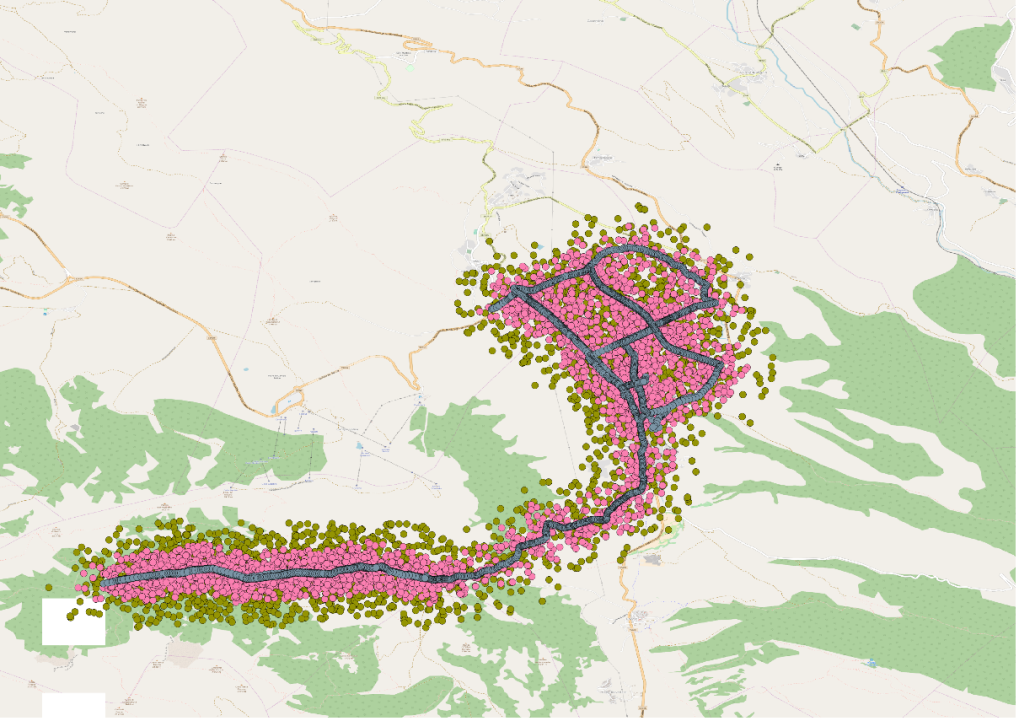
In this recipe, we applied three different mechanisms for noise-based location obfuscation: Rand, N-Rand, and Pinwheel, defining PostgreSQL functions in PLPGSQL for each method. We used one of the functions in a trigger in order to automatically alter the incoming data, so that no changes would need to be made on the application on the user's side. In addition, we showed the impact of noise comparing two versions of the altered data, so we can better appreciate the impact of the configuration noise settings
In the following recipes, we will look at an implementation of a private information retrieval-based LPPM.
Private information retrieval (PIR) LPPMs provide location privacy by mapping the spatial context to provide a private way to query a service without releasing any location information that could be obtained by third parties.
PIR-based methods can be classified as cryptography-based or hardware-based, according to [9]. Hardware-based methods use a special kind of secure coprocessor (SC) that acts as securely protected spaces in which the PIR query is processed in a non-decipherable way, as in [10]. Cryptography-based techniques only use logic resources, and do not require a special physical disposition on either the server or client-side.
In [10], the authors present a hybrid technique that uses a cloaking method through various-size grid Hilbert curves to limit the search domain of a generic cryptography-based PIR algorithm; however, the PIR processing on the database is still expensive, as shown in their experiments, and it is not practical for a user-defined level of privacy. This is because the method does not allow the cloaking grid cell size to be specified by the user, nor can it be changed once the whole grid has been calculated; in other words, no new PoIs can be added to the system. Other techniques can be found in [12].
PIR can also be combined with other techniques to increase the level of privacy. One type of compatible LPPM is the dummy query-based technique, where a set of random fake or dummy queries are generated for arbitrary locations within the greater search area (city, county, state, for example) [13], [14]. The purpose of this is to hide the one that the user actually wants to send.
The main disadvantage of the dummy query technique is the overall cost of sending and processing a large number of requests for both the user and the server sides. In addition, one of the queries will contain the original exact location and point of interest of the user, so the original trajectory could still be traced based on the query records from a user - especially if no intelligence is applied when generating the dummies. There are improvements to this method discussed in [15], where rather than sending each point on a separate query, all the dummy and real locations are sent along with the location interest specified by the user. In [16], the authors propose a method to avoid the random generation of points for each iteration, which should reduce the possibility of detecting the trend in real points; but this technique requires a lot of resources from the device when generating trajectories for each dummy path, generates separate queries per path, and still reveals the user's location.
The LPPM presented as an example in this book is MaPIR – a Map-based PIR [17]. This is a method that applies a mapping technique to provide a common language for the user and server, and that is also capable of providing redundant answers to single queries without overhead on the server-side, which, in turn, can improve response time due to a reduction in its use of geographical queries.
This technique creates a redundant geographical mapping of a certain area that uses the actual coordinate of the PoI to generate IDs on a different search scale. In the MaPIR paper, the decimal digit of the coordinate that will be used for the query. Near the Equator, each digit can be approximated to represent a certain distance, as shown in the following figure:
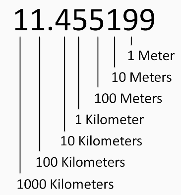
This can be generalized by saying that nearby locations will appear close at larger scales (closer to the integer portion of the location), but not necessarily in smaller ones. It could also show relatively far away points as though they were closer, if they share the same set of digits (nth digit of latitude and nth digit of longitude).
Once the digits have been obtained, depending on the selected scale, a mapping technique is needed to reduce the number to a single ID. On paper, a simple pseudo-random function is applied to reduce the two-dimensional domain to a one-dimensional one:
ID(Lat_Nth, Lon_Nth) = (((Lat_Nth + 1) * (Lon_Nth + 1)) mod p) - 1
In the preceding equation, we can see that p is the next prime number to the maximum desired ID. Given that for the paper the maximum ID was 9, the value of p is 11. After applying this function, the final map looks as follows:
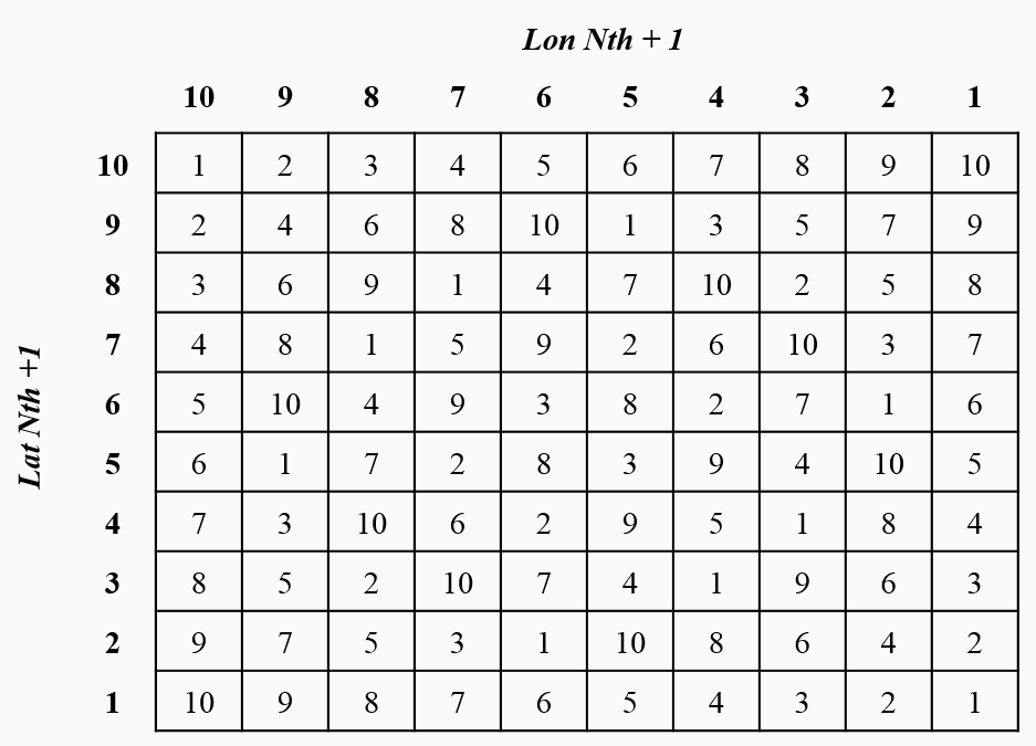
The following figure shows a sample PoI ID that represents a restaurant located at 10.964824,-74.804778. The final mapping grid cells will be 2, 6, and 1, using the scales k = 3, 2, and 1 respectively.
This information can be stored on a specific table in the database, or as the DBA determined best for the application:
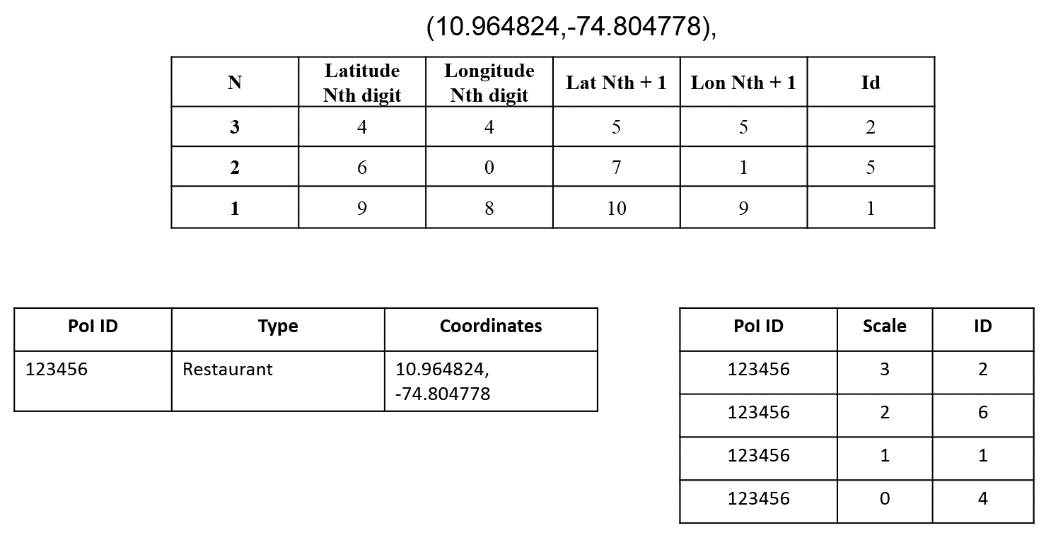
Based on this structure, a query generated by a user will need to define the scale of search (within 100 m, 1 km, and so on), the type of business they are looking for, and the grid cell they are located. The server will receive the parameters and look for all restaurants in the same cell ID as the user. The results will return all restaurants located in the cells with the same ID, even if they are not close to the user. Given that cells are indistinguishable, an attacker that gains access to the server's log will only see that a user was in 1 of 10 cell IDs. Of course, some of the IDs may fall in inhabitable areas (such as in a forest or lake), but some level of redundancy will always be present.
In this recipe, we will focus on the implementation of the MaPIR technique as an example of a PIR and dummy query-based LPPM. For this, a small dataset of supermarkets is loaded on the database as PoIs. These points will be processed and stored as explained in MaPIR, and then queried by a user.
The dataset was obtained from the Colombian open data platform Datos Abiertos at the following link:
The points in the dataset are presented in the following figure:
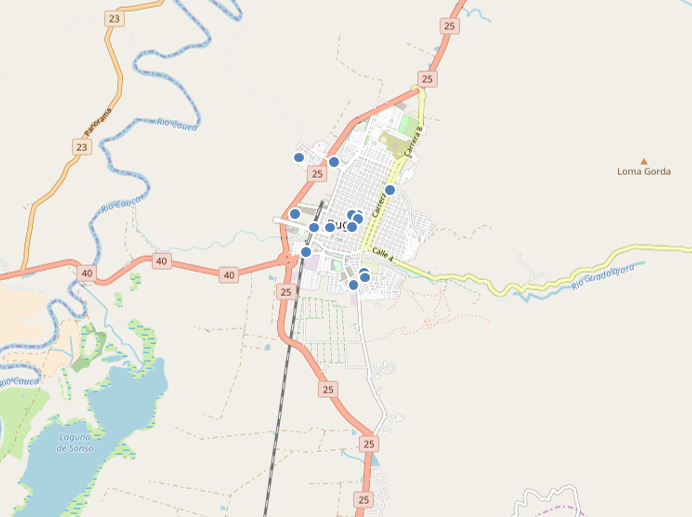
In the preceding recipe, we created temporary tables to store original data, as well as tables containing MaPIR information to be queried later by users. The following steps allow other users to access those tables:
CREATE TABLE chp12.supermarkets (
sup_id serial,
the_geom geometry(Point,4326),
latitude numeric,
longitude numeric,
PRIMARY KEY (sup_id)
);
CREATE TABLE chp12.supermarkets_mapir (
sup_id int REFERENCES chp12.supermarkets (sup_id),
cellid int,
levelid int
);
CREATE OR REPLACE FUNCTION __trigger_supermarkets_after_insert(
) RETURNS trigger AS $__$
DECLARE
tempcelliD integer;
BEGIN
FOR i IN -2..6
LOOP
tempcellid = mod((mod(CAST(TRUNC(ABS(NEW.latitude)*POWER(10,i))
as int),10)+1) * (mod(CAST(TRUNC(ABS(NEW.longitude)*POWER(10,i))
as int),10)+1), 11)-1;
INSERT INTO chp12.supermarkets_mapir (sup_id, cellid, levelid)
VALUES (NEW.sup_id, tempcellid, i);
END LOOP;
Return NEW;
END;
$__$ LANGUAGE plpgsql;
CREATE TRIGGER supermarkets_after_insert
AFTER INSERT ON chp12.supermarkets FOR EACH ROW
EXECUTE PROCEDURE __trigger_supermarkets_after_insert ();
INSERT INTO chp12.supermarkets (the_geom, longitude, latitude) VALUES
(ST_GEOMFROMTEXT('POINT(-76.304202 3.8992)',4326),
-76.304202, 3.8992),
(ST_GEOMFROMTEXT('POINT(-76.308476 3.894591)',4326),
-76.308476, 3.894591),
(ST_GEOMFROMTEXT('POINT(-76.297893 3.890615)',4326),
-76.297893, 3.890615),
(ST_GEOMFROMTEXT('POINT(-76.299017 3.901726)',4326),
-76.299017, 3.901726),
(ST_GEOMFROMTEXT('POINT(-76.292027 3.909094)',4326),
-76.292027, 3.909094),
(ST_GEOMFROMTEXT('POINT(-76.299687 3.888735)',4326),
-76.299687, 3.888735),
(ST_GEOMFROMTEXT('POINT(-76.307102 3.899181)',4326),
-76.307102, 3.899181),
(ST_GEOMFROMTEXT('POINT(-76.310342 3.90145)',4326),
-76.310342, 3.90145),
(ST_GEOMFROMTEXT('POINT(-76.297366 3.889721)',4326),
-76.297366, 3.889721),
(ST_GEOMFROMTEXT('POINT(-76.293296 3.906171)',4326),
-76.293296, 3.906171),
(ST_GEOMFROMTEXT('POINT(-76.300154 3.901235)',4326),
-76.300154, 3.901235),
(ST_GEOMFROMTEXT('POINT(-76.299755 3.899361)',4326),
-76.299755, 3.899361),
(ST_GEOMFROMTEXT('POINT(-76.303509 3.911253)',4326),
-76.303509, 3.911253),
(ST_GEOMFROMTEXT('POINT(-76.300152 3.901175)',4326),
-76.300152, 3.901175),
(ST_GEOMFROMTEXT('POINT(-76.299286 3.900895)',4326),
-76.299286, 3.900895),
(ST_GEOMFROMTEXT('POINT(-76.309937 3.912021)',4326),
-76.309937, 3.912021);
SELECT * FROM supermarkets_mapir WHERE sup_id = 8;
The result of the query is shown in the following table:
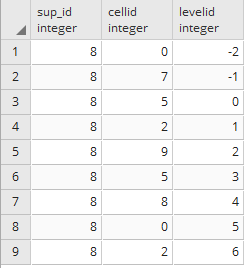
SELECT sm.the_geom AS the_geom
FROM chp12.supermarkets_mapir AS smm, chp12.supermarkets AS sm
WHERE smm.levelid = 2 AND smm.cellid = 9 AND smm.sup_id = sm.sup_id;
Note that there is no need for any geographical information in the query anymore, because the mapping was done during the pre-processing stage. This reduces the query time, because it does not require the use of complex internal functions to determine distance; however, mapping cannot guarantee that all nearby results will be returned, as results in adjacent cells with different IDs may not appear. In the following figure, you can see that the supermarkets from the previous query (in black) do not include some of the supermarkets that are near the user's location (in white near the arrow). Some possible counter-measures can be applied to tackle this, such as double-mapping some of the elements close to the edges of the grid cells:
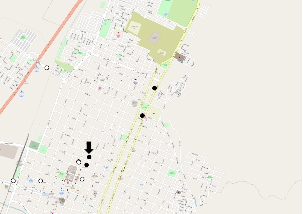
In this recipe, we implemented an LPPM that uses PIR and a dummy query called MaPIR. It created a mapping function for points of interest that allowed us to query using different scales. It also included redundancy in the answer, providing privacy protection, as it did not reveal the actual location of the user.
The process required for calculating the mapping of a dataset should be stored in a table that will be used for a user’s queries. In the MaPIR paper, it was shown that despite the multiple results, the execution time of the MaPIR queries took less than half the time, compared to the geopraphical queries based on distance.
European Union Directive on Privacy and Electronic Communications, 2002.
J. Krumm, Inference Attacks on Location Tracks, in Pervasive Computing. Springer, 2007, pp. 127-143.
M. A. Labrador, A. J. Perez, and P. Wightman. Location-based Information Systems: Developing Real-time Tracking Applications. Boca Raton: CRC Press, 2011.
M. Duckham and L. Kulik, A Formal Model of Obfuscation and Negotiation for Location Privacy, in Pervasive Computing. Springer, 2005, pp. 152-170.
P. Wightman, W. Coronell, D. Jabba, M. Jimeno, and M. Labrador, Evaluation of Location Obfuscation Techniques for Privacy in Location-based Information Systems, in Communications (LATINCOM), 2011 IEEE Latin-American Conference on, pp. 1-6.
P. Wightman, M. Zurbarán, E. Zurek, A. Salazar, D. Jabba, and M. Jimeno, θ-Rand: Random Noise-based Location Obfuscation Based on Circle Sectors, in IEEE International Symposium on Industrial Electronics and Applications (ISIEA) on, 2013.
P. Wightman, M. Zurbarán, and A. Santander, High Variability Geographical Obfuscation for Location Privacy, 2013 47th International Carnahan Conference on Security Technology (ICCST), Medellin, 2013, pp. 1-6.
A. Labrador, P. Wightman, A. Santander, D. Jabba, M. Jimeno, Tis-Bad: A Time Series-Based Deobfuscation Algorithm, in Investigación e Innovación en Ingenierías. Universidad Simón Bolívar. Vol. 3 (1), pp. 1 - 8. 2015.
A. Khoshgozaran, H. Shirani-Mehr, and C. Shahabi, SPIRAL: A Scalable Private Information Retrieval Approach to Location Privacy, in Mobile Data Management Workshops, 2008. MDMW 2008. Ninth International Conference on, pp. 55-62.
G. Ghinita, P. Kalnis, A. Khoshgozaran, C. Shahabi, and K. Tan, Private queries in location-based services: Anonymizers are not necessary, in Proceedings of the 2008 ACM SIGMOD International Conference on Management of Data, pp. 121-132.
D. Quercia, I. Leontiadis, L. McNamara, C. Mascolo, and J. Crowcroft, SpotME if you can: Randomized Responses for Location Obfuscation on Mobile Phones, in Distributed Computing Systems (ICDCS), 2011 31st International Conference on, 2011, pp. 363-372.
H. Kido, Y. Yanagisawa, and T. Satoh, An Anonymous Communication Technique using Dummies for Location-based Services, in Pervasive Services, 2005. ICPS '05. Proceedings. International Conference on, pp. 88-97.
H. Lu, C. S. Jensen, and M. L. Yiu, Pad: Privacy-area aware, dummy-based location privacy in mobile services, in Proceedings of the Seventh ACM International Workshop on Data Engineering for Wireless and Mobile Access, pp. 16-23.
P. Shankar, V. Ganapathy, and L. Iftode (2009, September), Privately Querying Location-based Services with sybilquery. In Proceedings of the 11th international conference on Ubiquitous computing, 2009, pp. 31-40.
If you enjoyed this book, you may be interested in these other books by Packt:
Mastering PostGIS
Dominik Mikiewicz, Michal Mackiewicz, Tomasz Nycz
ISBN: 978-1-78439-164-5
Please share your thoughts on this book with others by leaving a review on the site that you bought it from. If you purchased the book from Amazon, please leave us an honest review on this book's Amazon page. This is vital so that other potential readers can see and use your unbiased opinion to make purchasing decisions, we can understand what our customers think about our products, and our authors can see your feedback on the title that they have worked with Packt to create. It will only take a few minutes of your time, but is valuable to other potential customers, our authors, and Packt. Thank you!
Copyright © 2018 Packt Publishing
All rights reserved. No part of this book may be reproduced, stored in a retrieval system, or transmitted in any form or by any means, without the prior written permission of the publisher, except in the case of brief quotations embedded in critical articles or reviews.
Every effort has been made in the preparation of this book to ensure the accuracy of the information presented. However, the information contained in this book is sold without warranty, either express or implied. Neither the authors, nor Packt Publishing or its dealers and distributors, will be held liable for any damages caused or alleged to have been caused directly or indirectly by this book.
Packt Publishing has endeavored to provide trademark information about all of the companies and products mentioned in this book by the appropriate use of capitals. However, Packt Publishing cannot guarantee the accuracy of this information.
Commissioning Editor: Merint Mathew
Acquisition Editors: Nitin Dasan, Shriram Shekhar
Content Development Editor: Nikhil Borkar
Technical Editor: Subhalaxmi Nadar
Copy Editor: Safis Editing
Project Coordinator: Ulhas Kambali
Proofreader: Safis Editing
Indexer: Mariammal Chettiyar
Graphics: Tania Dutta
Production Coordinator: Shantanu Zagade
First published: January 2014
Second edition: March 2018
Production reference: 1270318
Published by Packt Publishing Ltd.
Livery Place
35 Livery Street
Birmingham
B3 2PB, UK.
ISBN 978-1-78829-932-9
Mapt is an online digital library that gives you full access to over 5,000 books and videos, as well as industry leading tools to help you plan your personal development and advance your career. For more information, please visit our website.
Spend less time learning and more time coding with practical eBooks and Videos from over 4,000 industry professionals
Improve your learning with Skill Plans built especially for you
Get a free eBook or video every month
Mapt is fully searchable
Copy and paste, print, and bookmark content
Did you know that Packt offers eBook versions of every book published, with PDF and ePub files available? You can upgrade to the eBook version at www.PacktPub.com and as a print book customer, you are entitled to a discount on the eBook copy. Get in touch with us at service@packtpub.com for more details.
At www.PacktPub.com, you can also read a collection of free technical articles, sign up for a range of free newsletters, and receive exclusive discounts and offers on Packt books and eBooks.
Mayra Zurbarán is a Colombian geogeek currently pursuing her PhD in geoprivacy. She has a BS in computer science from Universidad del Norte and is interested in the intersection of ethical location data management, free and open source software, and GIS. She is a Pythonista with a marked preference for the PostgreSQL database. Mayra is a member of the Geomatics and Earth Observation laboratory (GEOlab) at Politecnico di Milano and is also a contributor to the FOSS community.
Pedro M. Wightman is an associate professor at the Systems Engineering Department of Universidad del Norte, Barranquilla, Colombia. With a PhD in computer science from the University of South Florida, he's a researcher in location-based information systems, wireless sensor networks, and virtual and augmented reality, among other fields. Father of two beautiful and smart girls, he's also a rookie writer of short stories, science fiction fan, time travel enthusiast, and is worried about how to survive apocalyptic solar flares.
Paolo Corti is an environmental engineer with 20 years of experience in the GIS field, currently working as a Geospatial Engineer Fellow at the Center for Geographic Analysis at Harvard University. He is an advocate of open source geospatial technologies and Python, an OSGeo Charter member, and a member of the pycsw and GeoNode Project Steering Committees. He is a coauthor of the first edition of this book and the reviewer for the first and second editions of the Mastering QGIS book by Packt.
Stephen Vincent Mather has worked in the geospatial industry for 15 years, having always had a flair for geospatial analyses in general, especially those at the intersection of Geography and Ecology. His work in open-source geospatial databases started 5 years ago with PostGIS and he immediately began using PostGIS as an analytic tool, attempting a range of innovative and sometimes bleeding-edge techniques (although he admittedly prefers the cutting edge).
Thomas J Kraft is currently a Planning Technician at Cleveland Metroparks after beginning as a GIS intern in 2011. He graduated with Honors from Cleveland State University in 2012, majoring in Environmental Science with an emphasis on GIS. When not in front of a computer, he spends his weekends landscaping and in the outdoors in general.
Bborie Park has been breaking (and subsequently fixing) computers for most of his life. His primary interests involve developing end-to-end pipelines for spatial datasets. He is an active contributor to the PostGIS project and is a member of the PostGIS Steering Committee. He happily resides with his wife Nicole in the San Francisco Bay Area.
If you're interested in becoming an author for Packt, please visit authors.packtpub.com and apply today. We have worked with thousands of developers and tech professionals, just like you, to help them share their insight with the global tech community. You can make a general application, apply for a specific hot topic that we are recruiting an author for, or submit your own idea.
How close is the nearest hospital from my children's school? Where were the property crimes in my city for the last three months? What is the shortest route from my home to my office? What route should I prescribe for my company's delivery truck to maximize equipment utilization and minimize fuel consumption? Where should the next fire station be built to minimize response times?
People ask these questions, and others like them, every day all over this planet. Answering these questions requires a mechanism capable of thinking in two or more dimensions. Historically, desktop GIS applications were the only ones capable of answering these questions. This method—though completely functional—is not viable for the average person; most people do not need all the functionalities that these applications can offer, or they do not know how to use them. In addition, more and more location-based services offer the specific features that people use and are accessible even from their smartphones. Clearly, the massification of these services requires the support of a robust backend platform to process a large number of geographical operations.
Since scalability, support for large datasets, and a direct input mechanism are required or desired, most developers have opted to adopt spatial databases as their support platform. There are several spatial database software available, some proprietary and others open source. PostGIS is an open source spatial database software available, and probably the most accessible of all spatial database software.
PostGIS runs as an extension to provide spatial capabilities to PostgreSQL databases. In this capacity, PostGIS permits the inclusion of spatial data alongside data typically found in a database. By having all the data together, questions such as "What is the rank of all the police stations, after taking into account the distance for each response time?" are possible. New or enhanced capabilities are possible by building upon the core functions provided by PostGIS and the inherent extensibility of PostgreSQL. Furthermore, this book also includes an invitation to include location privacy protection mechanisms in new GIS applications and in location-based services so that users feel respected and not necessarily at risk for sharing their information, especially information as sensitive as their whereabouts.
PostGIS Cookbook, Second Edition uses a problem-solving approach to help you acquire a solid understanding of PostGIS. It is hoped that this book provides answers to some common spatial questions and gives you the inspiration and confidence to use and enhance PostGIS in finding solutions to challenging spatial problems.
This book is written for those who are looking for the best method to solve their spatial problems using PostGIS. These problems can be as simple as finding the nearest restaurant to a specific location, or as complex as finding the shortest and/or most efficient route from point A to point B.
For readers who are just starting out with PostGIS, or even with spatial datasets, this book is structured to help them become comfortable and proficient at running spatial operations in the database. For experienced users, the book provides opportunities to dive into advanced topics such as point clouds, raster map-algebra, and PostGIS programming.
Chapter 1, Moving Data In and Out of PostGIS, covers the processes available for importing and exporting spatial and non-spatial data to and from PostGIS. These processes include the use of utilities provided by PostGIS and by third parties, such as GDAL/OGR.
Chapter 2, Structures That Work, discusses how to organize PostGIS data using mechanisms available through PostgreSQL. These mechanisms are used to normalize potentially unclean and unstructured import data.
Chapter 3, Working with Vector Data – The Basics, introduces PostGIS operations commonly done on vectors, known as geometries and geographies in PostGIS. Operations covered include the processing of invalid geometries, determining relationships between geometries, and simplifying complex geometries.
Chapter 4, Working with Vector Data – Advanced Recipes, dives into advanced topics for analyzing geometries. You will learn how to make use of KNN filters to increase the performance of proximity queries, create polygons from LiDAR data, and compute Voronoi cells usable in neighborhood analyses.
Chapter 5, Working with Raster Data, presents a realistic workflow for operating on rasters in PostGIS. You will learn how to import a raster, modify the raster, conduct analysis on the raster, and export the raster in standard raster formats.
Chapter 6, Working with pgRouting, introduces the pgRouting extension, which brings graph traversal and analysis capabilities to PostGIS. The recipes in this chapter answer real-world questions of conditionally navigating from point A to point B and accurately modeling complex routes, such as waterways.
Chapter 7, Into the Nth Dimension, focuses on the tools and techniques used to process and analyze multidimensional spatial data in PostGIS, including LiDAR-sourced point clouds. Topics covered include the loading of point clouds into PostGIS, creating 2.5D and 3D geometries from point clouds, and the application of several photogrammetry principles.
Chapter 8, PostGIS Programming, shows how to use the Python language to write applications that operate on and interact with PostGIS. The applications written include methods to read and write external datasets to and from PostGIS, as well as a basic geocoding engine using OpenStreetMap datasets.
Chapter 9, PostGIS and the Web, presents the use of OGC and REST web services to deliver PostGIS data and services to the web. This chapter discusses providing OGC, WFS, and WMS services with MapServer and GeoServer, and consuming them from clients such as OpenLayers and Leaflet. It then shows how to build a web application with GeoDjango and how to include your PostGIS data in a Mapbox application.
Chapter 10, Maintenance, Optimization, and Performance Tuning, takes a step back from PostGIS and focuses on the capabilities of the PostgreSQL database server. By leveraging the tools provided by PostgreSQL, you can ensure the long-term viability of your spatial and non-spatial data, and maximize the performance of various PostGIS operations. In addition, it explores new features such as geospatial sharding and parallelism in PostgreSQL.
Chapter 11, Using Desktop Clients, tells you about how spatial data in PostGIS can be consumed and manipulated using various open source desktop GIS applications. Several applications are discussed so as to highlight the different approaches to interacting with spatial data and help you find the right tool for the task.
Chapter 12, Introduction to Location Privacy Protection Mechanisms, provides an introductory approximation to the concept of location privacy and presents the implementation of two different location privacy protection mechanisms that can be included in commercial applications to give a basic level of protection to the user's location data.
Before going further into this book, you will want to install latest versions of PostgreSQL and PostGIS (9.6 or 103 and 2.3 or 2.41, respectively). You may also want to install pgAdmin (1.18) if you prefer a graphical SQL tool. For most computing environments (Windows, Linux, macOS X), installers and packages include all required dependencies of PostGIS. The minimum required dependencies for PostGIS are PROJ.4, GEOS, libjson and GDAL.
A basic understanding of the SQL language is required to understand and adapt the code found in this book's recipes.
You can download the example code files for this book from your account at www.packtpub.com. If you purchased this book elsewhere, you can visit www.packtpub.com/support and register to have the files emailed directly to you.
You can download the code files by following these steps:
Once the file is downloaded, please make sure that you unzip or extract the folder using the latest version of:
The code bundle for the book is also hosted on GitHub at https://github.com/PacktPublishing/PostGIS-Cookbook-Second-Edition. In case there's an update to the code, it will be updated on the existing GitHub repository.
We also have other code bundles from our rich catalog of books and videos available at https://github.com/PacktPublishing/. Check them out!
We also provide a PDF file that has color images of the screenshots/diagrams used in this book. You can download it here: https://www.packtpub.com/sites/default/files/downloads/PostGISCookbookSecondEdition_ColorImages.pdf.
There are a number of text conventions used throughout this book.
CodeInText: Indicates code words in text, database table names, folder names, filenames, file extensions, pathnames, dummy URLs, user input, and Twitter handles. Here is an example: "We will import the firenews.csv file that stores a series of web news collected from various RSS feeds."
A block of code is set as follows:
SELECT ROUND(SUM(chp02.proportional_sum(ST_Transform(a.geom,3734), b.geom, b.pop))) AS population
FROM nc_walkzone AS a, census_viewpolygon as b
WHERE ST_Intersects(ST_Transform(a.geom, 3734), b.geom)
GROUP BY a.id;
When we wish to draw your attention to a particular part of a code block, the relevant lines or items are set in bold:
SELECT ROUND(SUM(chp02.proportional_sum(ST_Transform(a.geom,3734), b.geom, b.pop))) AS population
FROM nc_walkzone AS a, census_viewpolygon as b
WHERE ST_Intersects(ST_Transform(a.geom, 3734), b.geom)
GROUP BY a.id;
Any command-line input or output is written as follows:
> raster2pgsql -s 4322 -t 100x100 -F -I -C -Y C:\postgis_cookbook\data\chap5\PRISM\us_tmin_2012.*.asc chap5.prism | psql -d postgis_cookbook
Bold: Indicates a new term, an important word, or words that you see onscreen. For example, words in menus or dialog boxes appear in the text like this. Here is an example: "Clicking the Next button moves you to the next screen."
In this book, you will find several headings that appear frequently (Getting ready, How to do it..., How it works..., There's more..., and See also).
To give clear instructions on how to complete a recipe, use these sections as follows:
This section tells you what to expect in the recipe and describes how to set up any software or any preliminary settings required for the recipe.
This section contains the steps required to follow the recipe.
This section usually consists of a detailed explanation of what happened in the previous section.
This section consists of additional information about the recipe in order to make you more knowledgeable about the recipe.
This section provides helpful links to other useful information for the recipe.
Feedback from our readers is always welcome.
General feedback: Email feedback@packtpub.com and mention the book title in the subject of your message. If you have questions about any aspect of this book, please email us at questions@packtpub.com.
Errata: Although we have taken every care to ensure the accuracy of our content, mistakes do happen. If you have found a mistake in this book, we would be grateful if you would report this to us. Please visit www.packtpub.com/submit-errata, selecting your book, clicking on the Errata Submission Form link, and entering the details.
Piracy: If you come across any illegal copies of our works in any form on the internet, we would be grateful if you would provide us with the location address or website name. Please contact us at copyright@packtpub.com with a link to the material.
If you are interested in becoming an author: If there is a topic that you have expertise in and you are interested in either writing or contributing to a book, please visit authors.packtpub.com.
Please leave a review. Once you have read and used this book, why not leave a review on the site that you purchased it from? Potential readers can then see and use your unbiased opinion to make purchase decisions, we at Packt can understand what you think about our products, and our authors can see your feedback on their book. Thank you!
For more information about Packt, please visit packtpub.com.
In this chapter, we will cover:
PostGIS is an open source extension for the PostgreSQL database that allows support for geographic objects; throughout this book you will find recipes that will guide you step by step to explore the different functionalities it offers.
The purpose of the book is to become a useful tool for understanding the capabilities of PostGIS and how to apply them in no time. Each recipe presents a preparation stage, in order to organize your workspace with everything you may need, then the set of steps that you need to perform in order to achieve the main goal of the task, that includes all the external commands and SQL sentences you will need (which have been tested in Linux, Mac and Windows environments), and finally a small summary of the recipe. This book will go over a large set of common tasks in geographical information systems and location-based services, which makes it a must-have book in your technical library.
In this first chapter, we will show you a set of recipes covering different tools and methodologies to import and export geographic data from the PostGIS spatial database, given that pretty much every common action to perform in a GIS starts with inserting or exporting geospatial data.
There are a couple of alternative approaches to importing a Comma Separated Values (CSV) file, which stores attributes and geometries in PostGIS. In this recipe, we will use the approach of importing such a file using the PostgreSQL COPY command and a couple of PostGIS functions.
We will import the firenews.csv file that stores a series of web news collected from various RSS feeds related to forest fires in Europe in the context of the European Forest Fire Information System (EFFIS), available at http://effis.jrc.ec.europa.eu/.
For each news feed, there are attributes such as place name, size of the fire in hectares, URL, and so on. Most importantly, there are the x and y fields that give the position of the geolocalized news in decimal degrees (in the WGS 84 spatial reference system, SRID = 4326).
For Windows machines, it is necessary to install OSGeo4W, a set of open source geographical libraries that will allow the manipulation of the datasets. The link is: https://trac.osgeo.org/osgeo4w/
In addition, include the OSGeo4W and the Postgres binary folders in the Path environment variable to be able to execute the commands from any location in your PC.
The steps you need to follow to complete this recipe are as shown:
$ cd ~/postgis_cookbook/data/chp01/
$ head -n 5 firenews.csv
The output of the preceding command is as shown:
$ psql -U me -d postgis_cookbook
postgis_cookbook=> CREATE EXTENSION postgis;
postgis_cookbook=> CREATE SCHEMA chp01;
postgis_cookbook=> CREATE TABLE chp01.firenews
(
x float8,
y float8,
place varchar(100),
size float8,
update date,
startdate date,
enddate date,
title varchar(255),
url varchar(255),
the_geom geometry(POINT, 4326)
);
postgis_cookbook=> COPY chp01.firenews (
x, y, place, size, update, startdate,
enddate, title, url
) FROM '/tmp/firenews.csv' WITH CSV HEADER;
postgis_cookbook=> SELECT COUNT(*) FROM chp01.firenews;
The output of the preceding command is as follows:
postgis_cookbook=# SELECT f_table_name,
f_geometry_column, coord_dimension, srid, type
FROM geometry_columns where f_table_name = 'firenews';
The output of the preceding command is as follows:
In PostGIS 2.0, you can still use the AddGeometryColumn function if you wish; however, you need to set its use_typmod parameter to false.
postgis_cookbook=> UPDATE chp01.firenews
SET the_geom = ST_SetSRID(ST_MakePoint(x,y), 4326); postgis_cookbook=> UPDATE chp01.firenews
SET the_geom = ST_PointFromText('POINT(' || x || ' ' || y || ')',
4326);
postgis_cookbook=# SELECT place, ST_AsText(the_geom) AS wkt_geom
FROM chp01.firenews ORDER BY place LIMIT 5;
The output of the preceding comment is as follows:
postgis_cookbook=> CREATE INDEX idx_firenews_geom
ON chp01.firenews USING GIST (the_geom);
This recipe showed you how to load nonspatial tabular data (in CSV format) in PostGIS using the COPY PostgreSQL command.
After creating the table and copying the CSV file rows to the PostgreSQL table, you updated the geometric column using one of the geometry constructor functions that PostGIS provides (ST_MakePoint and ST_PointFromText for bi-dimensional points).
These geometry constructors (in this case, ST_MakePoint and ST_PointFromText) must always provide the spatial reference system identifier (SRID) together with the point coordinates to define the point geometry.
Each geometric field added in any table in the database is tracked with a record in the geometry_columns PostGIS metadata view. In the previous PostGIS version (< 2.0), the geometry_fields view was a table and needed to be manually updated, possibly with the convenient AddGeometryColumn function.
For the same reason, to maintain the updated geometry_columns view when dropping a geometry column or removing a spatial table in the previous PostGIS versions, there were the DropGeometryColumn and DropGeometryTable functions. With PostGIS 2.0 and newer, you don't need to use these functions any more, but you can safely remove the column or the table with the standard ALTER TABLE, DROP COLUMN, and DROP TABLE SQL commands.
In the last step of the recipe, you have created a spatial index on the table to improve performance. Please be aware that as in the case of alphanumerical database fields, indexes improve performances only when reading data using the SELECT command. In this case, you are making a number of updates on the table (INSERT, UPDATE, and DELETE); depending on the scenario, it could be less time consuming to drop and recreate the index after the updates.
As an alternative approach to the previous recipe, you will import a CSV file to PostGIS using the ogr2ogr GDAL command and the GDAL OGR virtual format. The Geospatial Data Abstraction Library (GDAL) is a translator library for raster geospatial data formats. OGR is the related library that provides similar capabilities for vector data formats.
This time, as an extra step, you will import only a part of the features in the file and you will reproject them to a different spatial reference system.
You will import the Global_24h.csv file to the PostGIS database from NASA's Earth Observing System Data and Information System (EOSDIS).
You can copy the file from the dataset directory of the book for this chapter.
This file represents the active hotspots in the world detected by the Moderate Resolution Imaging Spectroradiometer (MODIS) satellites in the last 24 hours. For each row, there are the coordinates of the hotspot (latitude, longitude) in decimal degrees (in the WGS 84 spatial reference system, SRID = 4326), and a series of useful fields such as the acquisition date, acquisition time, and satellite type, just to name a few.
You will import only the active fire data scanned by the satellite type marked as T (Terra MODIS), and you will project it using the Spherical Mercator projection coordinate system (EPSG:3857; it is sometimes marked as EPSG:900913, where the number 900913 represents Google in 1337 speak, as it was first widely used by Google Maps).
The steps you need to follow to complete this recipe are as follows:
$ cd ~/postgis_cookbook/data/chp01/
$ head -n 5 Global_24h.csv
The output of the preceding command is as follows:
<OGRVRTDataSource>
<OGRVRTLayer name="Global_24h">
<SrcDataSource>Global_24h.csv</SrcDataSource>
<GeometryType>wkbPoint</GeometryType>
<LayerSRS>EPSG:4326</LayerSRS>
<GeometryField encoding="PointFromColumns"
x="longitude" y="latitude"/>
</OGRVRTLayer>
</OGRVRTDataSource>
$ ogrinfo global_24h.vrt Global_24h -fid 1
The output of the preceding command is as follows:
You can also try to open the virtual layer with a desktop GIS supporting a GDAL/OGR virtual driver such as Quantum GIS (QGIS). In the following screenshot, the Global_24h layer is displayed together with the shapefile of the countries that you can find in the dataset directory of the book:
$ ogr2ogr -f PostgreSQL -t_srs EPSG:3857
PG:"dbname='postgis_cookbook' user='me' password='mypassword'"
-lco SCHEMA=chp01 global_24h.vrt -where "satellite='T'"
-lco GEOMETRY_NAME=the_geom
$ pg_dump -t chp01.global_24h --schema-only -U me postgis_cookbook
CREATE TABLE global_24h (
ogc_fid integer NOT NULL,
latitude character varying,
longitude character varying,
brightness character varying,
scan character varying,
track character varying,
acq_date character varying,
acq_time character varying,
satellite character varying,
confidence character varying,
version character varying,
bright_t31 character varying,
frp character varying,
the_geom public.geometry(Point,3857)
);
postgis_cookbook=# SELECT f_geometry_column, coord_dimension,
srid, type FROM geometry_columns
WHERE f_table_name = 'global_24h';
The output of the preceding command is as follows:
postgis_cookbook=# SELECT count(*) FROM chp01.global_24h;
The output of the preceding command is as follows:
postgis_cookbook=# SELECT ST_AsEWKT(the_geom)
FROM chp01.global_24h LIMIT 1;
The output of the preceding command is as follows:
As mentioned in the GDAL documentation:
GDAL supports the reading and writing of nonspatial tabular data stored as a CSV file, but we need to use a virtual format to derive the geometry of the layers from attribute columns in the CSV file (the longitude and latitude coordinates for each point). For this purpose, you need to at least specify in the driver the path to the CSV file (the SrcDataSource element), the geometry type (the GeometryType element), the spatial reference definition for the layer (the LayerSRS element), and the way the driver can derive the geometric information (the GeometryField element).
There are many other options and reasons for using OGR virtual formats; if you are interested in developing a better understanding, please refer to the GDAL documentation available at http://www.gdal.org/drv_vrt.html.
After a virtual format is correctly created, the original flat nonspatial dataset is spatially supported by GDAL and software-based on GDAL. This is the reason why we can manipulate these files with GDAL commands such as ogrinfo and ogr2ogr, and with desktop GIS software such as QGIS.
Once we have verified that GDAL can correctly read the features from the virtual driver, we can easily import them in PostGIS using the popular ogr2ogr command-line utility. The ogr2ogr command has a plethora of options, so refer to its documentation at http://www.gdal.org/ogr2ogr.html for a more in-depth discussion.
In this recipe, you have just seen some of these options, such as:
If you need to import a shapefile in PostGIS, you have at least a couple of options such as the ogr2ogr GDAL command, as you have seen previously, or the shp2pgsql PostGIS command.
In this recipe, you will load a shapefile in the database using the shp2pgsql command, analyze it with the ogrinfo command, and display it in QGIS desktop software.
The steps you need to follow to complete this recipe are as follows:
$ ogr2ogr global_24h.shp global_24h.vrt
$ shp2pgsql -G -I global_24h.shp
chp01.global_24h_geographic > global_24h.sql
$ head -n 20 global_24h.sql
The output of the preceding command is as follows:
$ psql -U me -d postgis_cookbook -f global_24h.sql
postgis_cookbook=# SELECT f_geography_column, coord_dimension,
srid, type FROM geography_columns
WHERE f_table_name = 'global_24h_geographic';
The output of the preceding command is as follows:
$ ogrinfo PG:"dbname='postgis_cookbook' user='me'
password='mypassword'" chp01.global_24h_geographic -fid 1
The output of the preceding command is as follows:
Now, open QGIS and try to add the new layer to the map. Navigate to Layer | Add Layer | Add PostGIS layers and provide the connection information, and then add the layer to the map as shown in the following screenshot:
The PostGIS command, shp2pgsql, allows the user to import a shapefile in the PostGIS database. Basically, it generates a PostgreSQL dump file that can be used to load data by running it from within PostgreSQL.
The SQL file will be generally composed of the following sections:
To get a complete list of the shp2pgsql command options and their meanings, just type the command name in the shell (or in the command prompt, if you are on Windows) and check the output.
There are GUI tools to manage data in and out of PostGIS, generally integrated into GIS desktop software such as QGIS. In the last chapter of this book, we will take a look at the most popular one.
In this recipe, you will use the popular ogr2ogr GDAL command for importing and exporting vector data from PostGIS.
Firstly, you will import a shapefile in PostGIS using the most significant options of the ogr2ogr command. Then, still using ogr2ogr, you will export the results of a spatial query performed in PostGIS to a couple of GDAL-supported vector formats.
The steps you need to follow to complete this recipe are as follows:
$ ogr2ogr -f PostgreSQL -sql "SELECT ISO2,
NAME AS country_name FROM wborders WHERE REGION=2" -nlt
MULTIPOLYGON PG:"dbname='postgis_cookbook' user='me'
password='mypassword'" -nln africa_countries
-lco SCHEMA=chp01 -lco GEOMETRY_NAME=the_geom wborders.shp
postgis_cookbook=# SELECTST_AsText(the_geom) AS the_geom, bright_t31
FROM chp01.global_24h
ORDER BY bright_t31 DESC LIMIT 100;
The output of the preceding command is as follows:
postgis_cookbook=# SELECT ST_AsText(f.the_geom)
AS the_geom, f.bright_t31, ac.iso2, ac.country_name
FROM chp01.global_24h as f
JOIN chp01.africa_countries as ac
ON ST_Contains(ac.the_geom, ST_Transform(f.the_geom, 4326))
ORDER BY f.bright_t31 DESCLIMIT 100;
The output of the preceding command is as follows:
You will now export the result of this query to a vector format supported by GDAL, such as GeoJSON, in the WGS 84 spatial reference using ogr2ogr:
$ ogr2ogr -f GeoJSON -t_srs EPSG:4326 warmest_hs.geojson
PG:"dbname='postgis_cookbook' user='me' password='mypassword'" -sql "
SELECT f.the_geom as the_geom, f.bright_t31,
ac.iso2, ac.country_name
FROM chp01.global_24h as f JOIN chp01.africa_countries as ac
ON ST_Contains(ac.the_geom, ST_Transform(f.the_geom, 4326))
ORDER BY f.bright_t31 DESC LIMIT 100"
$ ogr2ogr -t_srs EPSG:4326 -f CSV -lco GEOMETRY=AS_XY
-lco SEPARATOR=TAB warmest_hs.csv PG:"dbname='postgis_cookbook'
user='me' password='mypassword'" -sql "
SELECT f.the_geom, f.bright_t31,
ac.iso2, ac.country_name
FROM chp01.global_24h as f JOIN chp01.africa_countries as ac
ON ST_Contains(ac.the_geom, ST_Transform(f.the_geom, 4326))
ORDER BY f.bright_t31 DESC LIMIT 100"
GDAL is an open source library that comes together with several command-line utilities, which let the user translate and process raster and vector geodatasets into a plethora of formats. In the case of vector datasets, there is a GDAL sublibrary for managing vector datasets named OGR (therefore, when talking about vector datasets in the context of GDAL, we can also use the expression OGR dataset).
When you are working with an OGR dataset, two of the most popular OGR commands are ogrinfo, which lists many kinds of information from an OGR dataset, and ogr2ogr, which converts the OGR dataset from one format to another.
It is possible to retrieve a list of the supported OGR vector formats using the -formats option on any OGR commands, for example, with ogr2ogr:
$ ogr2ogr --formats
The output of the preceding command is as follows:
Note that some formats are read-only, while others are read/write.
PostGIS is one of the supported read/write OGR formats, so it is possible to use the OGR API or any OGR commands (such as ogrinfo and ogr2ogr) to manipulate its datasets.
The ogr2ogr command has many options and parameters; in this recipe, you have seen some of the most notable ones such as -f to define the output format, -t_srs to reproject/transform the dataset, and -sql to define an (eventually spatial) query in the input OGR dataset.
When using ogrinfo and ogr2ogr together with the desired option and parameters, you have to define the datasets. When specifying a PostGIS dataset, you need a connection string that is defined as follows:
PG:"dbname='postgis_cookbook' user='me' password='mypassword'"
You can find more information about the ogrinfo and ogr2ogr commands on the GDAL website available at http://www.gdal.org.
If you need more information about the PostGIS driver, you should check its related documentation page available at http://www.gdal.org/drv_pg.html.
In many GIS workflows, there is a typical scenario where subsets of a PostGIS table must be deployed to external users in a filesystem format (most typically, shapefiles or a spatialite database). Often, there is also the reverse process, where datasets received from different users have to be uploaded to the PostGIS database.
In this recipe, we will simulate both of these data flows. You will first create the data flow for processing the shapefiles out of PostGIS, and then the reverse data flow for uploading the shapefiles.
You will do it using the power of bash scripting and the ogr2ogr command.
If you didn't follow all the other recipes, be sure to import the hotspots (Global_24h.csv) and the countries dataset (countries.shp) in PostGIS. The following is how to do it with ogr2ogr (you should import both the datasets in their original SRID, 4326, to make spatial operations faster):
$ ogr2ogr -f PostgreSQL PG:"dbname='postgis_cookbook'
user='me' password='mypassword'" -lco SCHEMA=chp01 global_24h.vrt
-lco OVERWRITE=YES -lco GEOMETRY_NAME=the_geom -nln hotspots
$ ogr2ogr -f PostgreSQL -sql "SELECT ISO2, NAME AS country_name
FROM wborders" -nlt MULTIPOLYGON PG:"dbname='postgis_cookbook'
user='me' password='mypassword'" -nln countries
-lco SCHEMA=chp01 -lco OVERWRITE=YES
-lco GEOMETRY_NAME=the_geom wborders.shp
The steps you need to follow to complete this recipe are as follows:
postgis_cookbook=> SELECT c.country_name, MIN(c.iso2)
as iso2, count(*) as hs_count FROM chp01.hotspots as hs
JOIN chp01.countries as c ON ST_Contains(c.the_geom, hs.the_geom)
GROUP BY c.country_name ORDER BY c.country_name;
The output of the preceding command is as follows:
$ ogr2ogr -f CSV hs_countries.csv
PG:"dbname='postgis_cookbook' user='me' password='mypassword'"
-lco SCHEMA=chp01 -sql "SELECT c.country_name, MIN(c.iso2) as iso2,
count(*) as hs_count FROM chp01.hotspots as hs
JOIN chp01.countries as c ON ST_Contains(c.the_geom, hs.the_geom)
GROUP BY c.country_name ORDER BY c.country_name"
postgis_cookbook=> COPY (SELECT c.country_name, MIN(c.iso2) as iso2,
count(*) as hs_count FROM chp01.hotspots as hs
JOIN chp01.countries as c ON ST_Contains(c.the_geom, hs.the_geom)
GROUP BY c.country_name ORDER BY c.country_name)
TO '/tmp/hs_countries.csv' WITH CSV HEADER;
#!/bin/bash
while IFS="," read country iso2 hs_count
do
echo "Generating shapefile $iso2.shp for country
$country ($iso2) containing $hs_count features."
ogr2ogr out_shapefiles/$iso2.shp
PG:"dbname='postgis_cookbook' user='me' password='mypassword'"
-lco SCHEMA=chp01 -sql "SELECT ST_Transform(hs.the_geom, 4326),
hs.acq_date, hs.acq_time, hs.bright_t31
FROM chp01.hotspots as hs JOIN chp01.countries as c
ON ST_Contains(c.the_geom, ST_Transform(hs.the_geom, 4326))
WHERE c.iso2 = '$iso2'" done < hs_countries.csv
chmod 775 export_shapefiles.sh
mkdir out_shapefiles
$ ./export_shapefiles.sh
Generating shapefile AL.shp for country
Albania (AL) containing 66 features.
Generating shapefile DZ.shp for country
Algeria (DZ) containing 361 features.
...
Generating shapefile ZM.shp for country
Zambia (ZM) containing 1575 features.
Generating shapefile ZW.shp for country
Zimbabwe (ZW) containing 179 features.
@echo off
for /f "tokens=1-3 delims=, skip=1" %%a in (hs_countries.csv) do (
echo "Generating shapefile %%b.shp for country %%a
(%%b) containing %%c features"
ogr2ogr .\out_shapefiles\%%b.shp
PG:"dbname='postgis_cookbook' user='me' password='mypassword'"
-lco SCHEMA=chp01 -sql "SELECT ST_Transform(hs.the_geom, 4326),
hs.acq_date, hs.acq_time, hs.bright_t31
FROM chp01.hotspots as hs JOIN chp01.countries as c
ON ST_Contains(c.the_geom, ST_Transform(hs.the_geom, 4326))
WHERE c.iso2 = '%%b'"
)
>mkdir out_shapefiles
>export_shapefiles.bat
"Generating shapefile AL.shp for country
Albania (AL) containing 66 features"
"Generating shapefile DZ.shp for country
Algeria (DZ) containing 361 features"
...
"Generating shapefile ZW.shp for country
Zimbabwe (ZW) containing 179 features"
postgis_cookbook=# CREATE TABLE chp01.hs_uploaded
(
ogc_fid serial NOT NULL,
acq_date character varying(80),
acq_time character varying(80),
bright_t31 character varying(80),
iso2 character varying,
upload_datetime character varying,
shapefile character varying,
the_geom geometry(POINT, 4326),
CONSTRAINT hs_uploaded_pk PRIMARY KEY (ogc_fid)
);
$ brew install findutils
#!/bin/bash
for f in `find out_shapefiles -name \*.shp -printf "%f\n"`
do
echo "Importing shapefile $f to chp01.hs_uploaded PostGIS
table..." #, ${f%.*}"
ogr2ogr -append -update -f PostgreSQL
PG:"dbname='postgis_cookbook' user='me'
password='mypassword'" out_shapefiles/$f
-nln chp01.hs_uploaded -sql "SELECT acq_date, acq_time,
bright_t31, '${f%.*}' AS iso2, '`date`' AS upload_datetime,
'out_shapefiles/$f' as shapefile FROM ${f%.*}"
done
$ chmod 775 import_shapefiles.sh
$ ./import_shapefiles.sh
Importing shapefile DO.shp to chp01.hs_uploaded PostGIS table
...
Importing shapefile ID.shp to chp01.hs_uploaded PostGIS table
...
Importing shapefile AR.shp to chp01.hs_uploaded PostGIS table
......
Now, go to step 14.
@echo off
for %%I in (out_shapefiles\*.shp*) do (
echo Importing shapefile %%~nxI to chp01.hs_uploaded
PostGIS table...
ogr2ogr -append -update -f PostgreSQL
PG:"dbname='postgis_cookbook' user='me'
password='password'" out_shapefiles/%%~nxI
-nln chp01.hs_uploaded -sql "SELECT acq_date, acq_time,
bright_t31, '%%~nI' AS iso2, '%date%' AS upload_datetime,
'out_shapefiles/%%~nxI' as shapefile FROM %%~nI" )
>import_shapefiles.bat
Importing shapefile AL.shp to chp01.hs_uploaded PostGIS table...
Importing shapefile AO.shp to chp01.hs_uploaded PostGIS table...
Importing shapefile AR.shp to chp01.hs_uploaded PostGIS table......
postgis_cookbook=# SELECT upload_datetime,
shapefile, ST_AsText(wkb_geometry)
FROM chp01.hs_uploaded WHERE ISO2='AT';
The output of the preceding command is as follows:
$ ogrinfo PG:"dbname='postgis_cookbook' user='me'
password='mypassword'"
chp01.hs_uploaded -where "iso2='AT'"
The output of the preceding command is as follows:
You could implement both the data flows (processing shapefiles out from PostGIS, and then into it again) thanks to the power of the ogr2ogr GDAL command.
You have been using this command in different forms and with the most important input parameters in other recipes, so you should now have a good understanding of it.
Here, it is worth mentioning the way OGR lets you export the information related to the current datetime and the original shapefile name to the PostGIS table. Inside the import_shapefiles.sh (Linux, OS X) or the import_shapefiles.bat (Windows) scripts, the core is the line with the ogr2ogr command (here is the Linux version):
ogr2ogr -append -update -f PostgreSQL PG:"dbname='postgis_cookbook' user='me' password='mypassword'" out_shapefiles/$f -nln chp01.hs_uploaded -sql "SELECT acq_date, acq_time, bright_t31, '${f%.*}' AS iso2, '`date`' AS upload_datetime, 'out_shapefiles/$f' as shapefile FROM ${f%.*}"
Thanks to the -sql option, you can specify the two additional fields, getting their values from the system date command and the filename that is being iterated from the script.
In this recipe, you will export a PostGIS table to a shapefile using the pgsql2shp command that is shipped with any PostGIS distribution.
The steps you need to follow to complete this recipe are as follows:
$ shp2pgsql -I -d -s 4326 -W LATIN1 -g the_geom countries.shp
chp01.countries > countries.sql
$ psql -U me -d postgis_cookbook -f countries.sql
$ ogr2ogr -f PostgreSQL PG:"dbname='postgis_cookbook' user='me'
password='mypassword'"
-lco SCHEMA=chp01 countries.shp -nlt MULTIPOLYGON -lco OVERWRITE=YES
-lco GEOMETRY_NAME=the_geom
postgis_cookbook=> SELECT subregion,
ST_Union(the_geom) AS the_geom, SUM(pop2005) AS pop2005
FROM chp01.countries GROUP BY subregion;
$ pgsql2shp -f subregions.shp -h localhost -u me -P mypassword
postgis_cookbook "SELECT MIN(subregion) AS subregion,
ST_Union(the_geom) AS the_geom, SUM(pop2005) AS pop2005
FROM chp01.countries GROUP BY subregion;" Initializing... Done (postgis major version: 2). Output shape: Polygon Dumping: X [23 rows].
You have exported the results of a spatial query to a shapefile using the pgsql2shp PostGIS command. The spatial query you have used aggregates fields using the SUM PostgreSQL function for summing country populations in the same subregion, and the ST_Union PostGIS function to aggregate the corresponding geometries as a geometric union.
The pgsql2shp command allows you to export PostGIS tables and queries to shapefiles. The options you need to specify are quite similar to the ones you use to connect to PostgreSQL with psql. To get a full list of these options, just type pgsql2shp in your command prompt and read the output.
In this recipe, you will import OpenStreetMap (OSM) data to PostGIS using the osm2pgsql command.
You will first download a sample dataset from the OSM website, and then you will import it using the osm2pgsql command.
You will add the imported layers in GIS desktop software and generate a view to get subdatasets, using the hstore PostgreSQL additional module to extract features based on their tags.
We need the following in place before we can proceed with the steps required for the recipe:
$ sudo apt-get install osm2pgsql
$ osm2pgsqlosm2pgsql SVN version 0.80.0 (32bit id space)
postgres=# CREATE DATABASE rome OWNER me;
postgres=# \connect rome;
rome=# create extension postgis;
$ sudo apt-get update
$ sudo apt-get install postgresql-contrib-9.6
$ psql -U me -d romerome=# CREATE EXTENSION hstore;
The steps you need to follow to complete this recipe are as follows:
$ osm2pgsql -d rome -U me --hstore map.osm
osm2pgsql SVN version 0.80.0 (32bit id space)Using projection
SRS 900913 (Spherical Mercator)Setting up table:
planet_osm_point...All indexes on planet_osm_polygon created
in 1sCompleted planet_osm_polygonOsm2pgsql took 3s overall
rome=# SELECT f_table_name, f_geometry_column,
coord_dimension, srid, type FROM geometry_columns;
The output of the preceding command is shown here:
rome=# CREATE VIEW rome_trees AS SELECT way, tags
FROM planet_osm_polygon WHERE (tags -> 'landcover') = 'trees';
OpenStreetMap is a popular collaborative project for creating a free map of the world. Every user participating in the project can edit data; at the same time, it is possible for everyone to download those datasets in .osm datafiles (an XML format) under the terms of the Open Data Commons Open Database License (ODbL) at the time of writing.
The osm2pgsql command is a command-line tool that can import .osm datafiles (eventually zipped) to the PostGIS database. To use the command, it is enough to give the PostgreSQL connection parameters and the .osm file to import.
It is possible to import only features that have certain tags in the spatial database, as defined in the default.style configuration file. You can decide to comment in or out the OSM tagged features that you would like to import, or not, from this file. The command by default exports all the nodes and ways to linestring, point, and geometry PostGIS geometries.
It is highly recommended to enable hstore support in the PostgreSQL database and use the -hstore option of osm2pgsql when importing the data. Having enabled this support, the OSM tags for each feature will be stored in a hstore PostgreSQL data type, which is optimized for storing (and retrieving) sets of key/values pairs in a single field. This way, it will be possible to query the database as follows:
SELECT way, tags FROM planet_osm_polygon WHERE (tags -> 'landcover') = 'trees';
PostGIS 2.0 now has full support for raster datasets, and it is possible to import raster datasets using the raster2pgsql command.
In this recipe, you will import a raster file to PostGIS using the raster2pgsql command. This command, included in any PostGIS distribution from version 2.0 onward, is able to generate an SQL dump to be loaded in PostGIS for any GDAL raster-supported format (in the same fashion that the shp2pgsql command does for shapefiles).
After loading the raster to PostGIS, you will inspect it both with SQL commands (analyzing the raster metadata information contained in the database), and with the gdalinfo command-line utility (to understand the way the input raster2pgsql parameters have been reflected in the PostGIS import process).
You will finally open the raster in a desktop GIS and try a basic spatial query, mixing vector and raster tables.
We need the following in place before we can proceed with the steps required for the recipe:
$ shp2pgsql -I -d -s 4326 -W LATIN1 -g the_geom countries.shp
chp01.countries > countries.sql
$ psql -U me -d postgis_cookbook -f countries.sql
The steps you need to follow to complete this recipe are as follows:
$ gdalinfo worldclim/tmax09.bil
Driver: EHdr/ESRI .hdr Labelled
Files: worldclim/tmax9.bil
worldclim/tmax9.hdr
Size is 2160, 900
Coordinate System is:
GEOGCS[""WGS 84"",
DATUM[""WGS_1984"",
SPHEROID[""WGS 84"",6378137,298.257223563,
AUTHORITY[""EPSG"",""7030""]],
TOWGS84[0,0,0,0,0,0,0],
AUTHORITY[""EPSG"",""6326""]],
PRIMEM[""Greenwich"",0,
AUTHORITY[""EPSG"",""8901""]],
UNIT[""degree"",0.0174532925199433,
AUTHORITY[""EPSG"",""9108""]],
AUTHORITY[""EPSG"",""4326""]]
Origin = (-180.000000000000057,90.000000000000000)
Pixel Size = (0.166666666666667,-0.166666666666667)
Corner Coordinates:
Upper Left (-180.0000000, 90.0000000) (180d 0'' 0.00""W, 90d
0'' 0.00""N)
Lower Left (-180.0000000, -60.0000000) (180d 0'' 0.00""W, 60d
0'' 0.00""S)
Upper Right ( 180.0000000, 90.0000000) (180d 0'' 0.00""E, 90d
0'' 0.00""N)
Lower Right ( 180.0000000, -60.0000000) (180d 0'' 0.00""E, 60d
0'' 0.00""S)
Center ( 0.0000000, 15.0000000) ( 0d 0'' 0.00""E, 15d
0'' 0.00""N)
Band 1 Block=2160x1 Type=Int16, ColorInterp=Undefined
Min=-153.000 Max=441.000
NoData Value=-9999
$ raster2pgsql -I -C -F -t 100x100 -s 4326
worldclim/tmax01.bil chp01.tmax01 > tmax01.sql
$ psql -d postgis_cookbook -U me -f tmax01.sql
If you are in Linux, you may pipe the two commands in a unique line:
$ raster2pgsql -I -C -M -F -t 100x100 worldclim/tmax01.bil
chp01.tmax01 | psql -d postgis_cookbook -U me -f tmax01.sql
$ pg_dump -t chp01.tmax01 --schema-only -U me postgis_cookbook
...
CREATE TABLE tmax01 (
rid integer NOT NULL,
rast public.raster,
filename text,
CONSTRAINT enforce_height_rast CHECK (
(public.st_height(rast) = 100)
),
CONSTRAINT enforce_max_extent_rast CHECK (public.st_coveredby
(public.st_convexhull(rast), ''0103...''::public.geometry)
),
CONSTRAINT enforce_nodata_values_rast CHECK (
((public._raster_constraint_nodata_values(rast)
)::numeric(16,10)[] = ''{0}''::numeric(16,10)[])
),
CONSTRAINT enforce_num_bands_rast CHECK (
(public.st_numbands(rast) = 1)
),
CONSTRAINT enforce_out_db_rast CHECK (
(public._raster_constraint_out_db(rast) = ''{f}''::boolean[])
),
CONSTRAINT enforce_pixel_types_rast CHECK (
(public._raster_constraint_pixel_types(rast) =
''{16BUI}''::text[])
),
CONSTRAINT enforce_same_alignment_rast CHECK (
(public.st_samealignment(rast, ''01000...''::public.raster)
),
CONSTRAINT enforce_scalex_rast CHECK (
((public.st_scalex(rast))::numeric(16,10) =
0.166666666666667::numeric(16,10))
),
CONSTRAINT enforce_scaley_rast CHECK (
((public.st_scaley(rast))::numeric(16,10) =
(-0.166666666666667)::numeric(16,10))
),
CONSTRAINT enforce_srid_rast CHECK ((public.st_srid(rast) = 0)),
CONSTRAINT enforce_width_rast CHECK ((public.st_width(rast) = 100))
);
postgis_cookbook=# SELECT * FROM raster_columns;
postgis_cookbook=# SELECT count(*) FROM chp01.tmax01;
The output of the preceding command is as follows:
count
-------
198
(1 row)
gdalinfo PG":host=localhost port=5432 dbname=postgis_cookbook
user=me password=mypassword schema='chp01' table='tmax01'"
gdalinfo PG":host=localhost port=5432 dbname=postgis_cookbook
user=me password=mypassword schema='chp01' table='tmax01' mode=2"
$ ogr2ogr temp_grid.shp PG:"host=localhost port=5432
dbname='postgis_cookbook' user='me' password='mypassword'"
-sql "SELECT rid, filename, ST_Envelope(rast) as the_geom
FROM chp01.tmax01"
SELECT * FROM (
SELECT c.name, ST_Value(t.rast,
ST_Centroid(c.the_geom))/10 as tmax_jan FROM chp01.tmax01 AS t
JOIN chp01.countries AS c
ON ST_Intersects(t.rast, ST_Centroid(c.the_geom))
) AS foo
ORDER BY tmax_jan LIMIT 10;
The output is as follows:
The raster2pgsql command is able to load any raster formats supported by GDAL in PostGIS. You can have a format list supported by your GDAL installation by typing the following command:
$ gdalinfo --formats
In this recipe, you have been importing one raster file using some of the most common raster2pgsql options:
$ raster2pgsql -I -C -F -t 100x100 -s 4326 worldclim/tmax01.bil chp01.tmax01 > tmax01.sql
The -I option creates a GIST spatial index for the raster column. The -C option will create the standard set of constraints after the rasters have been loaded. The -F option will add a column with the filename of the raster that has been loaded. This is useful when you are appending many raster files to the same PostGIS raster table. The -s option sets the raster's SRID.
If you decide to include the -t option, then you will cut the original raster into tiles, each inserted as a single row in the raster table. In this case, you decided to cut the raster into 100 x 100 tiles, resulting in 198 table rows in the raster table.
Another important option is -R, which will register the raster as out-of-db; in such a case, only the metadata will be inserted in the database, while the raster will be out of the database.
The raster table contains an identifier for each row, the raster itself (eventually one of its tiles, if using the -t option), and eventually the original filename, if you used the -F option, as in this case.
You can analyze the PostGIS raster using SQL commands or the gdalinfo command. Using SQL, you can query the raster_columns view to get the most significant raster metadata (spatial reference, band number, scale, block size, and so on).
With gdalinfo, you can access the same information, using a connection string with the following syntax:
gdalinfo PG":host=localhost port=5432 dbname=postgis_cookbook user=me password=mypassword schema='chp01' table='tmax01' mode=2"
The mode parameter is not influential if you loaded the whole raster as a single block (for example, if you did not specify the -t option). But, as in the use case of this recipe, if you split it into tiles, gdalinfo will see each tile as a single subdataset with the default behavior (mode=1). If you want GDAL to consider the raster table as a unique raster dataset, you have to specify the mode option and explicitly set it to 2.
This recipe will guide you through the importing of multiple rasters at a time.
You will first import some different single band rasters to a unique single band raster table using the raster2pgsql command.
Then, you will try an alternative approach, merging the original single band rasters in a virtual raster, with one band for each of the original rasters, and then load the multiband raster to a raster table. To accomplish this, you will use the GDAL gdalbuildvrt command and then load the data to PostGIS with raster2pgsql.
Be sure to have all the original raster datasets you have been using for the previous recipe.
The steps you need to follow to complete this recipe are as follows:
$ raster2pgsql -d -I -C -M -F -t 100x100 -s 4326
worldclim/tmax*.bil chp01.tmax_2012 > tmax_2012.sql
$ psql -d postgis_cookbook -U me -f tmax_2012.sql
postgis_cookbook=# SELECT r_raster_column, srid,
ROUND(scale_x::numeric, 2) AS scale_x,
ROUND(scale_y::numeric, 2) AS scale_y, blocksize_x,
blocksize_y, num_bands, pixel_types, nodata_values, out_db
FROM raster_columns where r_table_schema='chp01'
AND r_table_name ='tmax_2012';
SELECT rid, (foo.md).*
FROM (SELECT rid, ST_MetaData(rast) As md
FROM chp01.tmax_2012) As foo;
The output of the preceding command is as shown here:
If you now query the table, you would be able to derive the month for each raster row only from the original_file column. In the table, you have imported 198 distinct records (rasters) for each of the 12 original files (we divided them into 100 x 100 blocks, if you remember). Test this with the following query:
postgis_cookbook=# SELECT COUNT(*) AS num_raster,
MIN(filename) as original_file FROM chp01.tmax_2012
GROUP BY filename ORDER BY filename;
SELECT REPLACE(REPLACE(filename, 'tmax', ''), '.bil', '') AS month,
(ST_VALUE(rast, ST_SetSRID(ST_Point(12.49, 41.88), 4326))/10) AS tmax
FROM chp01.tmax_2012
WHERE rid IN (
SELECT rid FROM chp01.tmax_2012
WHERE ST_Intersects(ST_Envelope(rast),
ST_SetSRID(ST_Point(12.49, 41.88), 4326))
)
ORDER BY month;
The output of the preceding command is as shown here:
$ gdalbuildvrt -separate tmax_2012.vrt worldclim/tmax*.bil
<VRTDataset rasterXSize="2160" rasterYSize="900">
<SRS>GEOGCS...</SRS>
<GeoTransform>
-1.8000000000000006e+02, 1.6666666666666699e-01, ...
</GeoTransform>
<VRTRasterBand dataType="Int16" band="1">
<NoDataValue>-9.99900000000000E+03</NoDataValue>
<ComplexSource>
<SourceFilename relativeToVRT="1">
worldclim/tmax01.bil
</SourceFilename>
<SourceBand>1</SourceBand>
<SourceProperties RasterXSize="2160" RasterYSize="900"
DataType="Int16" BlockXSize="2160" BlockYSize="1" />
<SrcRect xOff="0" yOff="0" xSize="2160" ySize="900" />
<DstRect xOff="0" yOff="0" xSize="2160" ySize="900" />
<NODATA>-9999</NODATA>
</ComplexSource>
</VRTRasterBand>
<VRTRasterBand dataType="Int16" band="2">
...
$ gdalinfo tmax_2012.vrt
The output of the preceding command is as follows:
...$ raster2pgsql -d -I -C -M -F -t 100x100 -s 4326 tmax_2012.vrt
chp01.tmax_2012_multi > tmax_2012_multi.sql
$ psql -d postgis_cookbook -U me -f tmax_2012_multi.sql
postgis_cookbook=# SELECT r_raster_column, srid, blocksize_x,
blocksize_y, num_bands, pixel_types
from raster_columns where r_table_schema='chp01'
AND r_table_name ='tmax_2012_multi';
postgis_cookbook=# SELECT
(ST_VALUE(rast, 1, ST_SetSRID(ST_Point(12.49, 41.88), 4326))/10)
AS jan,
(ST_VALUE(rast, 2, ST_SetSRID(ST_Point(12.49, 41.88), 4326))/10)
AS feb,
(ST_VALUE(rast, 3, ST_SetSRID(ST_Point(12.49, 41.88), 4326))/10)
AS mar,
(ST_VALUE(rast, 4, ST_SetSRID(ST_Point(12.49, 41.88), 4326))/10)
AS apr,
(ST_VALUE(rast, 5, ST_SetSRID(ST_Point(12.49, 41.88), 4326))/10)
AS may,
(ST_VALUE(rast, 6, ST_SetSRID(ST_Point(12.49, 41.88), 4326))/10)
AS jun,
(ST_VALUE(rast, 7, ST_SetSRID(ST_Point(12.49, 41.88), 4326))/10)
AS jul,
(ST_VALUE(rast, 8, ST_SetSRID(ST_Point(12.49, 41.88), 4326))/10)
AS aug,
(ST_VALUE(rast, 9, ST_SetSRID(ST_Point(12.49, 41.88), 4326))/10)
AS sep,
(ST_VALUE(rast, 10, ST_SetSRID(ST_Point(12.49, 41.88), 4326))/10)
AS oct,
(ST_VALUE(rast, 11, ST_SetSRID(ST_Point(12.49, 41.88), 4326))/10)
AS nov,
(ST_VALUE(rast, 12, ST_SetSRID(ST_Point(12.49, 41.88), 4326))/10)
AS dec
FROM chp01.tmax_2012_multi WHERE rid IN (
SELECT rid FROM chp01.tmax_2012_multi
WHERE ST_Intersects(rast, ST_SetSRID(ST_Point(12.49, 41.88), 4326))
);
The output of the preceding command is as follows:
You can import raster datasets in PostGIS using the raster2pgsql command.
In a scenario where you have multiple rasters representing the same variable at different times, as in this recipe, it makes sense to store all of the original rasters as a single table in PostGIS. In this recipe, we have the same variable (average maximum temperature) represented by a single raster for each month. You have seen that you could proceed in two different ways:
In this recipe, you will see a couple of main options for exporting PostGIS rasters to different raster formats. They are both provided as command-line tools, gdal_translate and gdalwarp, by GDAL.
You need the following in place before you can proceed with the steps required for the recipe:
$ gdalinfo --formats | grep -i postgis
The output of the preceding command is as follows:
PostGISRaster (rw): PostGIS Raster driver
$ gdalinfo PG:"host=localhost port=5432
dbname='postgis_cookbook' user='me' password='mypassword'
schema='chp01' table='tmax_2012_multi' mode='2'"
The steps you need to follow to complete this recipe are as follows:
$ gdal_translate -b 1 -b 2 -b 3 -b 4 -b 5 -b 6
PG:"host=localhost port=5432 dbname='postgis_cookbook'
user='me' password='mypassword' schema='chp01'
table='tmax_2012_multi' mode='2'" tmax_2012_multi_123456.tif
postgis_cookbook=# SELECT ST_Extent(the_geom)
FROM chp01.countries WHERE name = 'Italy';
The output of the preceding command is as follows:
$ gdal_translate -projwin 6.619 47.095 18.515 36.649
PG:"host=localhost port=5432 dbname='postgis_cookbook'
user='me' password='mypassword' schema='chp01'
table='tmax_2012_multi' mode='2'" tmax_2012_multi.tif
gdalwarp -t_srs EPSG:3857 PG:"host=localhost port=5432
dbname='postgis_cookbook' user='me' password='mypassword'
schema='chp01' table='tmax_2012_multi' mode='2'"
tmax_2012_multi_3857.tif
Both gdal_translate and gdalwarp can transform rasters from a PostGIS raster to all GDAL-supported formats. To get a complete list of the supported formats, you can use the --formats option of GDAL's command line as follows:
$ gdalinfo --formats
For both these GDAL commands, the default output format is GeoTiff; if you need a different format, you must use the -of option and assign to it one of the outputs produced by the previous command line.
In this recipe, you have tried some of the most common options for these two commands. As they are complex tools, you may try some more command options as a bonus step.
To get a better understanding, you should check out the excellent documentation on the GDAL website:
In this chapter, we will cover:
This chapter focuses on ways to structure data using the functionality provided by the combination of PostgreSQL and PostGIS. These will be useful approaches for structuring and cleaning up imported data, converting tabular data into spatial data on the fly when it is entered, and maintaining relationships between tables and datasets using functionality endemic to the powerful combination of PostgreSQL and PostGIS. There are three categories of techniques with which we will leverage these functionalities: automatic population and modification of data using views and triggers, object orientation using PostgreSQL table inheritance, and using PostGIS functions (stored procedures) to reconstruct and normalize problematic data.
Automatic population of data is where the chapter begins. By leveraging PostgreSQL views and triggers, we can create ad hoc and flexible solutions to create connections between and within the tables. By extension, and for more formal or structured cases, PostgreSQL provides table inheritance and table partitioning, which allow for explicit hierarchical relationships between tables. This can be useful in cases where an object inheritance model enforces data relationships that either represent the data better, thereby resulting in greater efficiencies, or reduce the administrative overhead of maintaining and accessing the datasets over time. With PostGIS extending that functionality, the inheritance can apply not just to the commonly used table attributes, but to leveraging spatial relationships between tables, resulting in greater query efficiency with very large datasets. Finally, we will explore PostGIS SQL patterns that provide table normalization of data inputs, so datasets that come from flat filesystems or are not normalized can be converted to a form we would expect in a database.
Views in PostgreSQL allow the ad hoc representation of data and data relationships in alternate forms. In this recipe, we'll be using views to allow for the automatic creation of point data based on tabular inputs. We can imagine a case where the input stream of data is non-spatial, but includes longitude and latitude or some other coordinates. We would like to automatically show this data as points in space.
We can create a view as a representation of spatial data pretty easily. The syntax for creating a view is similar to creating a table, for example:
CREATE VIEW viewname AS SELECT...
In the preceding command line, our SELECT query manipulates the data for us. Let's start with a small dataset. In this case, we will start with some random points, which could be real data.
First, we create the table from which the view will be constructed, as follows:
-- Drop the table in case it exists DROP TABLE IF EXISTS chp02.xwhyzed CASCADE; CREATE TABLE chp02.xwhyzed -- This table will contain numeric x, y, and z values ( x numeric, y numeric, z numeric ) WITH (OIDS=FALSE); ALTER TABLE chp02.xwhyzed OWNER TO me; -- We will be disciplined and ensure we have a primary key ALTER TABLE chp02.xwhyzed ADD COLUMN gid serial; ALTER TABLE chp02.xwhyzed ADD PRIMARY KEY (gid);
Now, let's populate this with the data for testing using the following query:
INSERT INTO chp02.xwhyzed (x, y, z) VALUES (random()*5, random()*7, random()*106); INSERT INTO chp02.xwhyzed (x, y, z) VALUES (random()*5, random()*7, random()*106); INSERT INTO chp02.xwhyzed (x, y, z) VALUES (random()*5, random()*7, random()*106); INSERT INTO chp02.xwhyzed (x, y, z) VALUES (random()*5, random()*7, random()*106);
Now, to create the view, we will use the following query:
-- Ensure we don't try to duplicate the view DROP VIEW IF EXISTS chp02.xbecausezed; -- Retain original attributes, but also create a point attribute from x and y CREATE VIEW chp02.xbecausezed AS SELECT x, y, z, ST_MakePoint(x,y) FROM chp02.xwhyzed;
Our view is really a simple transformation of the existing data using PostGIS's ST_MakePoint function. The ST_MakePoint function takes the input of two numbers to create a PostGIS point, and in this case our view simply uses our x and y values to populate the data. Any time there is an update to the table to add a new record with x and y values, the view will populate a point, which is really useful for data that is constantly being updated.
There are two disadvantages to this approach. The first is that we have not declared our spatial reference system in the view, so any software consuming these points will not know the coordinate system we are using, that is, whether it is a geographic (latitude/longitude) or a planar coordinate system. We will address this problem shortly. The second problem is that many software systems accessing these points may not automatically detect and use the spatial information from the table. This problem is addressed in the Using triggers to populate the geometry column recipe.
To address the first problem mentioned in the How it works... section, we can simply wrap our existing ST_MakePoint function in another function specifying the SRID as ST_SetSRID, as shown in the following query:
-- Ensure we don't try to duplicate the view DROP VIEW IF EXISTS chp02.xbecausezed; -- Retain original attributes, but also create a point attribute from x and y CREATE VIEW chp02.xbecausezed AS SELECT x, y, z, ST_SetSRID(ST_MakePoint(x,y), 3734) -- Add ST_SetSRID FROM chp02.xwhyzed;
In this recipe, we imagine that we have ever increasing data in our database, which needs spatial representation; however, in this case we want a hardcoded geometry column to be updated each time an insertion happens on the database, converting our x and y values to geometry as and when they are inserted into the database.
The advantage of this approach is that the geometry is then registered in the geometry_columns view, and therefore this approach works reliably with more PostGIS client types than creating a new geospatial view. This also provides the advantage of allowing for a spatial index that can significantly speed up a variety of queries.
We will start by creating another table of random points with x, y, and z values, as shown in the following query:
DROP TABLE IF EXISTS chp02.xwhyzed1 CASCADE; CREATE TABLE chp02.xwhyzed1 ( x numeric, y numeric, z numeric ) WITH (OIDS=FALSE); ALTER TABLE chp02.xwhyzed1 OWNER TO me; ALTER TABLE chp02.xwhyzed1 ADD COLUMN gid serial; ALTER TABLE chp02.xwhyzed1 ADD PRIMARY KEY (gid); INSERT INTO chp02.xwhyzed1 (x, y, z) VALUES (random()*5, random()*7, random()*106); INSERT INTO chp02.xwhyzed1 (x, y, z) VALUES (random()*5, random()*7, random()*106); INSERT INTO chp02.xwhyzed1 (x, y, z) VALUES (random()*5, random()*7, random()*106); INSERT INTO chp02.xwhyzed1 (x, y, z) VALUES (random()*5, random()*7, random()*106);
Now we need a geometry column to populate. By default, the geometry column will be populated with null values. We populate a geometry column using the following query:
SELECT AddGeometryColumn ('chp02','xwhyzed1','geom',3734,'POINT',2);
We now have a column called geom with an SRID of 3734; that is, a point geometry type in two dimensions. Since we have x, y, and z data, we could, in principle, populate a 3D point table using a similar approach.
Since all the geometry values are currently null, we will populate them using an UPDATE statement as follows:
UPDATE chp02.xwhyzed1 SET the_geom = ST_SetSRID(ST_MakePoint(x,y), 3734);
The query here is simple when broken down. We update the xwhyzed1 table and set the the_geom column using ST_MakePoint, construct our point using the x and y columns, and wrap it in an ST_SetSRID function in order to apply the appropriate spatial reference information. So far, we have just set the table up. Now, we need to create a trigger in order to continue to populate this information once the table is in use. The first part of the trigger is a new populated geometry function using the following query:
CREATE OR REPLACE FUNCTION chp02.before_insertXYZ() RETURNS trigger AS $$ BEGIN if NEW.geom is null then NEW.geom = ST_SetSRID(ST_MakePoint(NEW.x,NEW.y), 3734); end if; RETURN NEW; END; $$ LANGUAGE 'plpgsql';
In essence, we have created a function that does exactly what we did manually: update the table's geometry column with the combination of ST_SetSRID and ST_MakePoint, but only to the new registers being inserted, and not to all the table.
While we have a function created, we have not yet applied it as a trigger to the table. Let us do that here as follows:
CREATE TRIGGER popgeom_insert
BEFORE INSERT ON chp02.xwhyzed1
FOR EACH ROW EXECUTE PROCEDURE chp02.before_insertXYZ();
Let's assume that the general geometry column update has not taken place yet, then the original five registers still have their geometry column in null. Now, once the trigger has been activated, any inserts into our table should be populated with new geometry records. Let us do a test insert using the following query:
INSERT INTO chp02.xwhyzed1 (x, y, z)
VALUES (random()*5, random()*7, 106),
(random()*5, random()*7, 107),
(random()*5, random()*7, 108),
(random()*5, random()*7, 109),
(random()*5, random()*7, 110);
Check the rows to verify that the geom columns are updated with the command:
SELECT * FROM chp02.xwhyzed1;
Or use pgAdmin:
After applying the general update, then all the registers will have a value on their geom column:
So far, we've implemented an insert trigger. What if the value changes for a particular row? In that case, we will require a separate update trigger. We'll change our original function to test the UPDATE case, and we'll use WHEN in our trigger to constrain updates to the column being changed.
Also, note that the following function is written with the assumption that the user wants to always update the changing geometries based on the changing values:
CREATE OR REPLACE FUNCTION chp02.before_insertXYZ()
RETURNS trigger AS
$$
BEGIN
if (TG_OP='INSERT') then
if (NEW.geom is null) then
NEW.geom = ST_SetSRID(ST_MakePoint(NEW.x,NEW.y), 3734);
end if;
ELSEIF (TG_OP='UPDATE') then
NEW.geom = ST_SetSRID(ST_MakePoint(NEW.x,NEW.y), 3734);
end if;
RETURN NEW;
END;
$$
LANGUAGE 'plpgsql';
CREATE TRIGGER popgeom_insert
BEFORE INSERT ON chp02.xwhyzed1
FOR EACH ROW EXECUTE PROCEDURE chp02.before_insertXYZ();
CREATE trigger popgeom_update
BEFORE UPDATE ON chp02.xwhyzed1
FOR EACH ROW
WHEN (OLD.X IS DISTINCT FROM NEW.X OR OLD.Y IS DISTINCT FROM
NEW.Y)
EXECUTE PROCEDURE chp02.before_insertXYZ();
An unusual and useful property of the PostgreSQL database is that it allows for object inheritance models as they apply to tables. This means that we can have parent/child relationships between tables and leverage that to structure the data in meaningful ways. In our example, we will apply this to hydrology data. This data can be points, lines, polygons, or more complex structures, but they have one commonality: they are explicitly linked in a physical sense and inherently related; they are all about water. Water/hydrology is an excellent natural system to model this way, as our ways of modeling it spatially can be quite mixed depending on scales, details, the data collection process, and a host of other factors.
The data we will be using is hydrology data that has been modified from engineering blue lines (see the following screenshot), that is, hydrologic data that is very detailed and is meant to be used at scales approaching 1:600. The data in its original application aided, as breaklines, in detailed digital terrain modeling.
While useful in itself, the data was further manipulated, separating the linear features from area features, with additional polygonization of the area features, as shown in the following screenshot:
Finally, the data was classified into basic waterway categories, as follows:
In addition, a process was undertaken to generate centerlines for polygon features such as streams, which are effectively linear features, as follows:
Hence, we have three separate but related datasets:
Now, let us look at the structure of the tabular data. Unzip the hydrology file from the book repository and go to that directory. The ogrinfo utility can help us with this, as shown in the following command:
> ogrinfo cuyahoga_hydro_polygon.shp -al -so
The output is as follows:
Executing this query on each of the shapefiles, we see the following fields that are common to all the shapefiles:
It is by understanding our common fields that we can apply inheritance to completely structure our data.
Now that we know our common fields, creating an inheritance model is easy. First, we will create a parent table with the fields common to all the tables, using the following query:
CREATE TABLE chp02.hydrology ( gid SERIAL PRIMARY KEY, "name" text, hyd_type text, geom_type text, the_geom geometry );
If you are paying attention, you will note that we also added a geometry field as all of our shapefiles implicitly have this commonality. With inheritance, every record inserted in any of the child tables will also be saved in our parent table, only these records will be stored without the extra fields specified for the child tables.
To establish inheritance for a given table, we need to declare only the additional fields that the child table contains using the following query:
CREATE TABLE chp02.hydrology_centerlines ( "length" numeric ) INHERITS (chp02.hydrology); CREATE TABLE chp02.hydrology_polygon ( area numeric, perimeter numeric ) INHERITS (chp02.hydrology); CREATE TABLE chp02.hydrology_linestring ( sinuosity numeric ) INHERITS (chp02.hydrology_centerlines);
Now, we are ready to load our data using the following commands:
If we view our parent table, we will see all the records in all the child tables. The following is a screenshot of fields in hydrology:
Compare that to the fields available in hydrology_linestring that will reveal specific fields of interest:
PostgreSQL table inheritance allows us to enforce essentially hierarchical relationships between tables. In this case, we leverage inheritance to allow for commonality between related datasets. Now, if we want to query data from these tables, we can query directly from the parent table as follows, depending on whether we want a mix of geometries or just a targeted dataset:
SELECT * FROM chp02.hydrology
From any of the child tables, we could use the following query:
SELECT * FROM chp02.hydrology_polygon
It is possible to extend this concept in order to leverage and optimize storage and querying by using the CHECK constrains in conjunction with inheritance. For more info, see the Extending inheritance – table partitioning recipe.
Table partitioning is an approach specific to PostgreSQL that extends inheritance to model tables that typically do not vary from each other in the available fields, but where the child tables represent logical partitioning of the data based on a variety of factors, be it time, value ranges, classifications, or in our case, spatial relationships. The advantages of partitioning include improved query performance due to smaller indexes and targeted scans of data, bulk loads, and deletes that bypass the costs of vacuuming. It can thus be used to put commonly used data on faster and more expensive storage, and the remaining data on slower and cheaper storage. In combination with PostGIS, we get the novel power of spatial partitioning, which is a really powerful feature for large datasets.
We could use many examples of large datasets that could benefit from partitioning. In our case, we will use a contour dataset. Contours are useful ways to represent terrain data, as they are well established and thus commonly interpreted. Contours can also be used to compress terrain data into linear representations, thus allowing it to be shown in conjunction with other data easily.
The problem is, the storage of contour data can be quite expensive. Two-foot contours for a single US county can take 20 to 40 GB, and storing such data for a larger area such as a region or nation can become quite prohibitive from the standpoint of accessing the appropriate portion of the dataset in a performant way.
The first step in this case may be to prepare the data. If we had a monolithic contour table called cuy_contours_2, we could choose to clip the data to a series of rectangles that will serve as our table partitions; in this case, chp02.contour_clip, using the following query:
CREATE TABLE chp02.contour_2_cm_only AS
SELECT contour.elevation, contour.gid, contour.div_10, contour.div_20, contour.div_50,
contour.div_100, cc.id, ST_Intersection(contour.the_geom, cc.the_geom) AS the_geom FROM
chp02.cuy_contours_2 AS contour, chp02.contour_clip as cc
WHERE ST_Within(contour.the_geom,cc.the_geom
OR
ST_Crosses(contour.the_geom,cc.the_geom);
We are performing two tests here in our query. We are using ST_Within, which tests whether a given contour is entirely within our area of interest. If so, we perform an intersection; the resultant geometry should just be the geometry of the contour.
The ST_Crosses function checks whether the contour crosses the boundary of the geometry we are testing. This should capture all the geometries lying partially inside and partially outside our areas. These are the ones that we will truly intersect to get the resultant shape.
In our case, it is easier and we don't require this step. Our contour shapes are already individual shapefiles clipped to rectangular boundaries, as shown in the following screenshot:
Since the data is already clipped into the chunks needed for our partitions, we can just continue to create the appropriate partitions.
Much like with inheritance, we start by creating our parent table using the following query:
CREATE TABLE chp02.contours ( gid serial NOT NULL, elevation integer, __gid double precision, the_geom geometry(MultiLineStringZM,3734), CONSTRAINT contours_pkey PRIMARY KEY (gid) ) WITH ( OIDS=FALSE );
Here again, we maintain our constraints, such as PRIMARY KEY, and specify the geometry type (MultiLineStringZM), not because these will propagate to the child tables, but for any client software accessing the parent table to anticipate such constraints.
Now we may begin to create tables that inherit from our parent table. In the process, we will create a CHECK constraint specifying the limits of our associated geometry using the following query:
CREATE TABLE chp02.contour_N2260630 (CHECK
(ST_CoveredBy(the_geom,ST_GeomFromText
('POLYGON((2260000, 630000, 2260000 635000, 2265000 635000,
2265000 630000, 2260000 630000))',3734)
)
)) INHERITS (chp02.contours);
We can complete the table structure for partitioning the contours with similar CREATE TABLE queries for our remaining tables, as follows:
CREATE TABLE chp02.contour_N2260635 (CHECK
(ST_CoveredBy(the_geom,ST_GeomFromText
('POLYGON((2260000 635000, 2260000 640000,
2265000 640000, 2265000 635000, 2260000 635000))', 3734) )
)) INHERITS (chp02.contours); CREATE TABLE chp02.contour_N2260640 (CHECK
(ST_CoveredBy(the_geom,ST_GeomFromText
('POLYGON((2260000 640000, 2260000 645000, 2265000 645000,
2265000 640000, 2260000 640000))', 3734) )
)) INHERITS (chp02.contours); CREATE TABLE chp02.contour_N2265630 (CHECK
(ST_CoveredBy(the_geom,ST_GeomFromText
('POLYGON((2265000 630000, 2265000 635000, 2270000 635000,
2270000 630000, 2265000 630000))', 3734)
)
)) INHERITS (chp02.contours); CREATE TABLE chp02.contour_N2265635 (CHECK
(ST_CoveredBy(the_geom,ST_GeomFromText
('POLYGON((2265000 635000, 2265000 640000, 2270000 640000,
2270000 635000, 2265000 635000))', 3734) )
)) INHERITS (chp02.contours); CREATE TABLE chp02.contour_N2265640 (CHECK
(ST_CoveredBy(the_geom,ST_GeomFromText
('POLYGON((2265000 640000, 2265000 645000, 2270000 645000,
2270000 640000, 2265000 640000))', 3734) )
)) INHERITS (chp02.contours); CREATE TABLE chp02.contour_N2270630 (CHECK
(ST_CoveredBy(the_geom,ST_GeomFromText
('POLYGON((2270000 630000, 2270000 635000, 2275000 635000,
2275000 630000, 2270000 630000))', 3734) )
)) INHERITS (chp02.contours); CREATE TABLE chp02.contour_N2270635 (CHECK
(ST_CoveredBy(the_geom,ST_GeomFromText
('POLYGON((2270000 635000, 2270000 640000, 2275000 640000,
2275000 635000, 2270000 635000))', 3734) )
)) INHERITS (chp02.contours); CREATE TABLE chp02.contour_N2270640 (CHECK
(ST_CoveredBy(the_geom,ST_GeomFromText
('POLYGON((2270000 640000, 2270000 645000, 2275000 645000,
2275000 640000, 2270000 640000))', 3734) )
)) INHERITS (chp02.contours);
And now we can load our contours shapefiles found in the contours1 ZIP file into each of our child tables, using the following command, by replacing the filename. If we wanted to, we could even implement a trigger on the parent table, which would place each insert into its correct child table, though this might incur performance costs:
shp2pgsql -s 3734 -a -i -I -W LATIN1 -g the_geom N2265630 chp02.contour_N2265630 | psql -U me -d postgis_cookbook
The CHECK constraint in combination with inheritance is all it takes to build a table partitioning. In this case, we're using a bounding box as our CHECK constraint and simply inheriting the columns from the parent table. Now that we have this in place, queries against the parent table will check our CHECK constraints first before employing a query.
This also allows us to place any of our lesser-used contour tables on cheaper and slower storage, thus allowing for cost-effective optimizations of large datasets. This structure is also beneficial for rapidly changing data, as updates can be applied to an entire area; the entire table for that area can be efficiently dropped and repopulated without traversing across the dataset.
For more on table inheritance in general, particularly the flexibility associated with the usage of alternate columns in the child table, see the previous recipe, Structuring spatial data with table inheritance.
Often, data used in a spatial database is imported from other sources. As such, it may not be in a form that is useful for our current application. In such a case, it may be useful to write functions that will aid in transforming the data into a form that is more useful for our application. This is particularly the case when going from flat file formats, such as shapefiles, to relational databases such as PostgreSQL.
There are many structures that might serve as a proxy for relational stores in a shapefile. We will explore one here: a single field with delimited text for multiple relations. This is a not-too-uncommon hack to encode multiple relationships into a flat file. The other common approach is to create multiple fields to store what in a relational arrangement would be a single field.
The dataset we will be working with is a trails dataset that has linear extents for a set of trails in a park system. The data is the typical data that comes from the GIS world; as a flat shapefile, there are no explicit relational constructs in the data.
First, unzip the trails.zip file and use the command line to go into it, then load the data using the following command:
shp2pgsql -s 3734 -d -i -I -W LATIN1 -g the_geom trails chp02.trails | psql -U me -d postgis_cookbook
Looking at the linear data, we have some categories for the use type:
We want to retain this information as well as the name. Unfortunately, the label_name field is a messy field with a variety of related names concatenated with an ampersand (&), as shown in the following query:
SELECT DISTINCT label_name FROM chp02.trails WHERE label_name LIKE '%&%' LIMIT 10;
It will return the following output:
This is where the normalization of our table will begin.
The first thing we need to do is find all the fields that don't have ampersands and use those as our unique list of available trails. In our case, we can do this, as every trail has at least one segment that is uniquely named and not associated with another trail name. This approach will not work with all datasets, so be careful in understanding your data before applying this approach to that data.
To select the fields ordered without ampersands, we use the following query:
SELECT DISTINCT label_name, res FROM chp02.trails WHERE label_name NOT LIKE '%&%' ORDER BY label_name, res;
It will return the following output:
Next, we want to search for all the records that match any of these unique trail names. This will give us the list of records that will serve as relations. The first step in doing this search is to append the percent (%) signs to our unique list in order to build a string on which we can search using a LIKE query:
SELECT '%' || label_name || '%' AS label_name, label_name as label, res FROM
(SELECT DISTINCT label_name, res
FROM chp02.trails
WHERE label_name NOT LIKE '%&%'
ORDER BY label_name, res
) AS label;
Finally, we'll use this in the context of a WITH block to do the normalization itself. This will provide us with a table of unique IDs for each segment in our first column, along with the associated label column. For good measure, we will do this as a CREATE TABLE procedure, as shown in the following query:
CREATE TABLE chp02.trails_names AS WITH labellike AS
(
SELECT '%' || label_name || '%' AS label_name, label_name as label, res FROM
(SELECT DISTINCT label_name, res
FROM chp02.trails
WHERE label_name NOT LIKE '%&%'
ORDER BY label_name, res
) AS label
)
SELECT t.gid, ll.label, ll.res
FROM chp02.trails AS t, labellike AS ll
WHERE t.label_name LIKE ll.label_name
AND
t.res = ll.res
ORDER BY gid;
If we view the first rows of the table created, trails_names, we have the following output with pgAdmin:
Now that we have a table of the relations, we need a table of the geometries associated with gid. This, in comparison, is quite easy, as shown in the following query:
CREATE TABLE chp02.trails_geom AS SELECT gid, the_geom FROM chp02.trails;
In this example, we have generated a unique list of possible records in conjunction with a search for the associated records, in order to build table relationships. In one table, we have the geometry and a unique ID of each spatial record; in another table, we have the names associated with each of those unique IDs. Now we can explicitly leverage those relationships.
First, we need to establish our unique IDs as primary keys, as follows:
ALTER TABLE chp02.trails_geom ADD PRIMARY KEY (gid);
Now we can use that PRIMARY KEY as a FOREIGN KEY in our trails_names table using the following query:
ALTER TABLE chp02.trails_names ADD FOREIGN KEY (gid) REFERENCES chp02.trails_geom(gid);
This step isn't strictly necessary, but does enforce referential integrity for queries such as the following:
SELECT geo.gid, geo.the_geom, names.label FROM chp02.trails_geom AS geo, chp02.trails_names AS names WHERE geo.gid = names.gid;
The output is as follows:
If we had multiple fields we wanted to normalize, we could write CREATE TABLE queries for each of them.
It is interesting to note that the approach framed in this recipe is not limited to cases where we have a delimited field. This approach can provide a relatively generic solution to the problem of normalizing flat files. For example, if we have a case where we have multiple fields to represent relational info, such as label1, label2, label3, or similar multiple attribute names for a single record, we can write a simple query to concatenate them together before feeding that info into our query.
Data from an external source can have issues in the table structure as well as in the topology, endemic to the geospatial data itself. Take, for example, the problem of data with overlapping polygons. If our dataset has polygons that overlap with internal overlays, then queries for area, perimeter, and other metrics may not produce predictable or consistent results.
There are a few approaches that can solve the problem of polygon datasets with internal overlays. The general approach presented here was originally proposed by Kevin Neufeld of Refractions Research.
Over the course of writing our query, we will also produce a solution for converting polygons to linestrings.
First, unzip the use_area.zip file and go into it using the command line; then, load the dataset using the following command:
shp2pgsql -s 3734 -d -i -I -W LATIN1 -g the_geom cm_usearea_polygon chp02.use_area | psql -U me -d postgis_cookbook
Now that the data is loaded into a table in the database, we can leverage PostGIS to flatten and get the union of the polygons, so that we have a normalized dataset. The first step in doing so using this approach will be to convert the polygons to linestrings. We can then link those linestrings and convert them back to polygons, representing the union of all the polygon inputs. We will perform the following tasks:
To convert polygons to linestrings, we'll need to extract just the portions of the polygons we want using ST_ExteriorRing, convert those parts to points using ST_DumpPoints, and then connect those points back into lines like a connect-the-dots coloring book using ST_MakeLine.
Breaking it down further, ST_ExteriorRing (the_geom) will grab just the outer boundary of our polygons. But ST_ExteriorRing returns polygons, so we need to take that output and create a line from it. The easiest way to do this is to convert it to points using ST_DumpPoints and then connect those points. By default, the Dump function returns an object called a geometry_dump, which is not just simple geometry, but the geometry in combination with an array of integers. The easiest way to return the geometry alone is the leverage object notation to extract just the geometry portion of geometry_dump, as follows:
(ST_DumpPoints(geom)).geom
Piecing the geometry back together with ST_ExteriorRing is done using the following query:
SELECT (ST_DumpPoints(ST_ExteriorRing(geom))).geom
This should give us a listing of points in order from the exterior rings of all the points from which we want to construct our lines using ST_MakeLine, as shown in the following query:
SELECT ST_MakeLine(geom) FROM ( SELECT (ST_DumpPoints(ST_ExteriorRing(geom))).geom) AS linpoints
Since the preceding approach is a process we may want to use in many other places, it might be prudent to create a function from this using the following query:
CREATE OR REPLACE FUNCTION chp02.polygon_to_line(geometry)
RETURNS geometry AS
$BODY$
SELECT ST_MakeLine(geom) FROM (
SELECT (ST_DumpPoints(ST_ExteriorRing((ST_Dump($1)).geom))).geom
) AS linpoints
$BODY$
LANGUAGE sql VOLATILE;
ALTER FUNCTION chp02.polygon_to_line(geometry)
OWNER TO me;
Now that we have the polygon_to_line function, we still need to force the linking of overlapping lines in our particular case. The ST_Union function will aid in this, as shown in the following query:
SELECT ST_Union(the_geom) AS geom FROM (
SELECT chp02.polygon_to_line(geom) AS geom FROM
chp02.use_area
) AS unioned;
Now let's convert linestrings back to polygons, and for this we can polygonize the result using ST_Polygonize, as shown in the following query:
SELECT ST_Polygonize(geom) AS geom FROM (
SELECT ST_Union(the_geom) AS geom FROM (
SELECT chp02.polygon_to_line(geom) AS geom FROM
chp02.use_area
) AS unioned
) as polygonized;
The ST_Polygonize function will create a single multi polygon, so we need to explode this into multiple single polygon geometries if we are to do anything useful with it. While we are at it, we might as well do the following within a CREATE TABLE statement:
CREATE TABLE chp02.use_area_alt AS (
SELECT (ST_Dump(the_geom)).geom AS the_geom FROM (
SELECT ST_Polygonize(the_geom) AS the_geom FROM (
SELECT ST_Union(the_geom) AS the_geom FROM (
SELECT chp02.polygon_to_line(the_geom) AS the_geom
FROM chp02.use_area
) AS unioned
) as polygonized
) AS exploded
);
We will be performing spatial queries against this geometry, so we should create an index in order to ensure our query performs well, as shown in the following query:
CREATE INDEX chp02_use_area_alt_the_geom_gist ON chp02.use_area_alt USING gist(the_geom);
In order to find the appropriate table information from the original geometry and apply that back to our resultant geometries, we will perform a point-in-polygon query. For that, we first need to calculate centroids on the resultant geometry:
CREATE TABLE chp02.use_area_alt_p AS
SELECT ST_SetSRID(ST_PointOnSurface(the_geom), 3734) AS
the_geom FROM
chp02.use_area_alt;
ALTER TABLE chp02.use_area_alt_p ADD COLUMN gid serial;
ALTER TABLE chp02.use_area_alt_p ADD PRIMARY KEY (gid);
And as always, create a spatial index using the following query:
CREATE INDEX chp02_use_area_alt_p_the_geom_gist ON chp02.use_area_alt_p USING gist(the_geom);
The centroids then structure our point-in-polygon (ST_Intersects) relationship between the original tabular information and resultant polygons, using the following query:
CREATE TABLE chp02.use_area_alt_relation AS
SELECT points.gid, cu.location FROM
chp02.use_area_alt_p AS points,
chp02.use_area AS cu
WHERE ST_Intersects(points.the_geom, cu.the_geom);
If we view the first rows of the table, we can see it links the identifier of points to their respective locations:
Our essential approach here is to look at the underlying topology of the geometry and reconstruct a topology that is non-overlapping, and then use the centroids of that new geometry to construct a query that establishes the relationship to the original data.
At this stage, we can optionally establish a framework for referential integrity using a foreign key, as follows:
ALTER TABLE chp02.use_area_alt_relation ADD FOREIGN KEY (gid) REFERENCES chp02.use_area_alt_p (gid);
PostgreSQL functions abound for the aggregation of tabular data, including sum, count, min, max, and so on. PostGIS as a framework does not explicitly have spatial equivalents of these, but this does not prevent us from building functions using the aggregate functions from PostgreSQL in concert with PostGIS's spatial functionality.
In this recipe, we will explore spatial summarization with the United States census data. The US census data, by nature, is aggregated data. This is done intentionally to protect the privacy of citizens. But when it comes to doing analyses with this data, the aggregate nature of the data can become problematic. There are some tricks to disaggregate data. Amongst the simplest of these is the use of a proportional sum, which we will do in this exercise.
The problem at hand is that a proposed trail has been drawn in order to provide services for the public. This example could apply to road construction or even finding sites for commercial properties for the purpose of provisioning services.
First, unzip the trail_census.zip file, then perform a quick data load using the following commands from the unzipped folder:
shp2pgsql -s 3734 -d -i -I -W LATIN1 -g the_geom census chp02.trail_census | psql -U me -d postgis_cookbook shp2pgsql -s 3734 -d -i -I -W LATIN1 -g the_geom trail_alignment_proposed_buffer chp02.trail_buffer | psql -U me -d postgis_cookbook shp2pgsql -s 3734 -d -i -I -W LATIN1 -g the_geom trail_alignment_proposed chp02.trail_alignment_prop | psql -U me -d postgis_cookbook
The preceding commands will produce the following outputs:
If we view the proposed trail in our favorite desktop GIS, we have the following:
In our case, we want to know the population within 1 mile of the trail, assuming that persons living within 1 mile of the trail are the ones most likely to use it, and thus most likely to be served by it.
To find out the population near this proposed trail, we overlay census block group population density information. Illustrated in the next screenshot is a 1-mile buffer around the proposed trail:
One of the things we might note about this census data is the wide range of census densities and census block group sizes. An approach to calculating the population would be to simply select all census blocks that intersect our area, as shown in the following screenshot:
This is a simple procedure that gives us an estimate of 130 to 288 people living within 1 mile of the trail, but looking at the shape of the selection, we can see that we are overestimating the population by taking the complete blocks in our estimate.
Similarly, if we just used the block groups whose centroids lay within 1 mile of our proposed trail alignment, we would underestimate the population.
Instead, we will make some useful assumptions. Block groups are designed to be moderately homogeneous within the block group population distribution. Assuming that this holds true for our data, we can assume that for a given block group, if 50% of the block group is within our target area, we can attribute half of the population of that block group to our estimate. Apply this to all our block groups, sum them, and we have a refined estimate that is likely to be better than pure intersects or centroid queries. Thus, we employ a proportional sum.
As the problem of a proportional sum is a generic problem, it could apply to many problems. We will write the underlying proportioning as a function. A function takes inputs and returns a value. In our case, we want our proportioning function to take two geometries, that is, the geometry of our buffered trail and block groups as well as the value we want proportioned, and we want it to return the proportioned value:
CREATE OR REPLACE FUNCTION chp02.proportional_sum(geometry, geometry, numeric) RETURNS numeric AS $BODY$ -- SQL here $BODY$ LANGUAGE sql VOLATILE;
Now, for the purpose of our calculation, for any given intersection of buffered area and block group, we want to find the proportion that the intersection is over the overall block group. Then this value should be multiplied by the value we want to scale.
In SQL, the function looks like the following query:
SELECT $3 * areacalc FROM (SELECT (ST_Area(ST_Intersection($1, $2)) / ST_Area($2)):: numeric AS areacalc ) AS areac;
The preceding query in its full form looks as follows:
CREATE OR REPLACE FUNCTION chp02.proportional_sum(geometry, geometry, numeric)
RETURNS numeric AS
$BODY$
SELECT $3 * areacalc FROM
(SELECT (ST_Area(ST_Intersection($1, $2))/ST_Area($2))::numeric AS areacalc
) AS areac
;
$BODY$
LANGUAGE sql VOLATILE;
Since we have written the query as a function, the query uses the SELECT statement to loop through all available records and give us a proportioned population. Astute readers will note that we have not yet done any work on summarization; we have only worked on the proportionality portion of the problem. We can do the summarization upon calling the function using PostgreSQL's built-in aggregate functions. What is neat about this approach is that we need not just apply a sum, but we could also calculate other aggregates such as min or max. In the following example, we will just apply a sum:
SELECT ROUND(SUM(chp02.proportional_sum(a.the_geom, b.the_geom, b.pop))) FROM chp02.trail_buffer AS a, chp02.trail_census as b WHERE ST_Intersects(a.the_geom, b.the_geom) GROUP BY a.gid;
The value returned is quite different (a population of 96,081), which is more likely to be accurate.
In this chapter, we will cover the following recipes:
In this chapter, you will work with a set of PostGIS functions and vector datasets. You will first take a look at how to use PostGIS with GPS data—you will import such datasets using ogr2ogr and then compose polylines from point geometries using the ST_MakeLine function.
Then, you will see how PostGIS helps you find and fix invalid geometries with functions such as ST_MakeValid, ST_IsValid, ST_IsValidReason, and ST_IsValidDetails.
You will then learn about one of the most powerful elements of a spatial database, spatial joins. PostGIS provides you with a rich set of operators, such as ST_Intersects, ST_Contains, ST_Covers, ST_Crosses, and ST_DWithin, for this purpose.
After that, you will use the ST_Simplify and ST_SimplifyPreverveTopology functions to simplify (generalize) geometries when you don't need too many details. While this function works well on linear geometries, topological anomalies may be introduced for polygonal ones. In such cases, you should consider using an external GIS tool such as GRASS.
You will then have a tour of PostGIS functions to make distance measurements—ST_Distance, ST_DistanceSphere, and ST_DistanceSpheroid are on the way.
One of the recipes explained in this chapter will guide you through the typical GIS workflow to merge polygons based on a common attribute; you will use the ST_Union function for this purpose.
You will then learn how to clip geometries using the ST_Intersection function, before deep diving into the PostGIS topology in the last recipe that was introduced in version 2.0.
In this recipe, you will work with GPS data. This kind of data is typically saved in a .gpx file. You will import a bunch of .gpx files to PostGIS from RunKeeper, a popular social network for runners.
If you have an account on RunKeeper, you can export your .gpx files and process them by following the instructions in this recipe. Otherwise, you can use the RunKeeper .gpx files included in the runkeeper-gpx.zip file located in the chp03 directory available in the code bundle for this book.
You will first create a bash script for importing the .gpx files to a PostGIS table, using ogr2ogr. After the import is completed, you will try to write a couple of SQL queries and test some very useful functions, such as ST_MakeLine to generate polylines from point geometries, ST_Length to compute distance, and ST_Intersects to perform a spatial join operation.
Extract the data/chp03/runkeeper-gpx.zip file to working/chp03/runkeeper_gpx. In case you haven't been through Chapter 1, Moving Data In and Out of PostGIS, be sure to have the countries dataset in the PostGIS database.
First, be sure of the format of the .gpx files that you need to import to PostGIS. Open one of them and check the file structure—each file must be in the XML format composed of just one <trk> element, which contains just one <trkseg> element, which contains many <trkpt> elements (the points stored from the runner's GPS device). Import these points to a PostGIS Point table:
postgis_cookbook=# create schema chp03;
postgis_cookbook=# CREATE TABLE chp03.rk_track_points
(
fid serial NOT NULL,
the_geom geometry(Point,4326),
ele double precision,
"time" timestamp with time zone,
CONSTRAINT activities_pk PRIMARY KEY (fid)
);
The following is the Linux version (name it working/chp03/import_gpx.sh):
#!/bin/bash
for f in `find runkeeper_gpx -name \*.gpx -printf "%f\n"`
do
echo "Importing gpx file $f to chp03.rk_track_points
PostGIS table..." #, ${f%.*}"
ogr2ogr -append -update -f PostgreSQL
PG:"dbname='postgis_cookbook' user='me'
password='mypassword'" runkeeper_gpx/$f
-nln chp03.rk_track_points
-sql "SELECT ele, time FROM track_points"
done
The following is the command for macOS (name it working/chp03/import_gpx.sh):
#!/bin/bash
for f in `find runkeeper_gpx -name \*.gpx `
do
echo "Importing gpx file $f to chp03.rk_track_points
PostGIS table..." #, ${f%.*}"
ogr2ogr -append -update -f PostgreSQL
PG:"dbname='postgis_cookbook' user='me'
password='mypassword'" $f
-nln chp03.rk_track_points
-sql "SELECT ele, time FROM track_points"
done
The following is the Windows version (name it working/chp03/import_gpx.bat):
@echo off
for %%I in (runkeeper_gpx\*.gpx*) do (
echo Importing gpx file %%~nxI to chp03.rk_track_points
PostGIS table...
ogr2ogr -append -update -f PostgreSQL
PG:"dbname='postgis_cookbook' user='me'
password='mypassword'" runkeeper_gpx/%%~nxI
-nln chp03.rk_track_points
-sql "SELECT ele, time FROM track_points"
)
$ chmod 775 import_gpx.sh
$ ./import_gpx.sh
Importing gpx file 2012-02-26-0930.gpx to chp03.rk_track_points
PostGIS table...
Importing gpx file 2012-02-29-1235.gpx to chp03.rk_track_points
PostGIS table...
...
Importing gpx file 2011-04-15-1906.gpx to chp03.rk_track_points
PostGIS table...
In Windows, just double-click on the .bat file or run it from the command prompt using the following command:
> import_gpx.bat
postgis_cookbook=# SELECT
ST_MakeLine(the_geom) AS the_geom,
run_date::date,
MIN(run_time) as start_time,
MAX(run_time) as end_time
INTO chp03.tracks
FROM (
SELECT the_geom,
"time"::date as run_date,
"time" as run_time
FROM chp03.rk_track_points
ORDER BY run_time
) AS foo GROUP BY run_date;
postgis_cookbook=# CREATE INDEX rk_track_points_geom_idx
ON chp03.rk_track_points USING gist(the_geom); postgis_cookbook=# CREATE INDEX tracks_geom_idx
ON chp03.tracks USING gist(the_geom);
postgis_cookbook=# SELECT
EXTRACT(year FROM run_date) AS run_year,
EXTRACT(MONTH FROM run_date) as run_month,
SUM(ST_Length(geography(the_geom)))/1000 AS distance
FROM chp03.tracks
GROUP BY run_year, run_month ORDER BY run_year, run_month;
(28 rows)
postgis_cookbook=# SELECT
c.country_name,
SUM(ST_Length(geography(t.the_geom)))/1000 AS run_distance
FROM chp03.tracks AS t
JOIN chp01.countries AS c
ON ST_Intersects(t.the_geom, c.the_geom)
GROUP BY c.country_name
ORDER BY run_distance DESC;
(4 rows)
The .gpx files store all the points' details in the WGS 84 spatial reference system; therefore, we created the rk_track_points table with SRID (4326).
After creating the rk_track_points table, we imported all of the .gpx files in the runkeeper_gpx directory using a bash script. The bash script iterates all of the files with the extension *.gpx in the runkeeper_gpx directory. For each of these files, the script runs the ogr2ogr command, importing the .gpx files to PostGIS using the GPX GDAL driver (for more details, go to http://www.gdal.org/drv_gpx.html).
In the GDAL's abstraction, a .gpx file is an OGR data source composed of several layers as follows:
In the .gpx files (OGR data sources), you have just the tracks and track_points layers. As a shortcut, you could have imported just the tracks layer using ogr2ogr, but you would need to start from the track_points layer in order to generate the tracks layer itself, using some PostGIS functions. This is why in the ogr2ogr section in the bash script, we imported to the rk_track_points PostGIS table the point geometries from the track_points layer, plus a couple of useful attributes, such as elevation and timestamp.
Once the records were imported, we fed a new polylines table named tracks using a subquery and selected all of the point geometries and their dates and times from the rk_track_points table, grouped by date and with the geometries aggregated using the ST_MakeLine function. This function was able to create linestrings from point geometries (for more details, go to http://www.postgis.org/docs/ST_MakeLine.html).
You should not forget to sort the points in the subquery by datetime; otherwise, you will obtain an irregular linestring, jumping from one point to the other and not following the correct order.
After loading the tracks table, we tested the two spatial queries.
At first, you got a month-by-month report of the total distance run by the runner. For this purpose, you selected all of the track records grouped by date (year and month), with the total distance obtained by summing up the lengths of the single tracks (obtained with the ST_Length function). To get the year and the month from the run_date function, you used the PostgreSQL EXTRACT function. Be aware that if you measure the distance using geometries in the WGS 84 system, you will obtain it in degree units. For this reason, you have to project the geometries to a planar metric system designed for the specific region from which the data will be projected.
For large-scale areas, such as in our case where we have points that span all around Europe, as shown in the last query results, a good option is to use the geography data type introduced with PostGIS 1.5. The calculations may be slower, but are much more accurate than in other systems. This is the reason why you cast the geometries to the geography data type before making measurements.
The last spatial query used a spatial join with the ST_Intersects function to get the name of the country for each track the runner ran (with the assumption that the runner didn't run cross-border tracks). Getting the total distance run per country is just a matter of aggregating the selection on the country_name field and aggregating the track distances with the PostgreSQL SUM operator.
You will often find invalid geometries in your PostGIS database. These invalid geometries could compromise the functioning of PostGIS itself and any external tool using it, such as QGIS and MapServer. PostGIS, being compliant with the OGC Simple Feature Specification, must manage and work with valid geometries.
Luckily, PostGIS 2.0 offers you the ST_MakeValid function, which together with the ST_IsValid, ST_IsValidReason, and ST_IsValidDetails functions, is the ideal toolkit for inspecting and fixing geometries within the database. In this recipe, you will learn how to fix a common case of invalid geometry.
Unzip the data/TM_WORLD_BORDERS-0.3.zip file into your working directory, working/chp3. Import the shapefile in PostGIS with the shp2pgsql command, as follows:
$ shp2pgsql -s 4326 -g the_geom -W LATIN1 -I TM_WORLD_BORDERS-0.3.shp chp03.countries > countries.sql $ psql -U me -d postgis_cookbook -f countries.sql
The steps you need to perform to complete this recipe are as follows:
postgis_cookbook=# SELECT gid, name, ST_IsValidReason(the_geom)
FROM chp03.countries
WHERE ST_IsValid(the_geom)=false;
(4 rows)
postgis_cookbook=# SELECT * INTO chp03.invalid_geometries FROM (
SELECT 'broken'::varchar(10) as status,
ST_GeometryN(the_geom, generate_series(
1, ST_NRings(the_geom)))::geometry(Polygon,4326)
as the_geom FROM chp03.countries
WHERE name = 'Russia') AS foo
WHERE ST_Intersects(the_geom,
ST_SetSRID(ST_Point(143.661926,49.31221), 4326));
ST_MakeValid requires GEOS 3.3.0 or higher; check whether or not your system supports it using the PostGIS_full_version function as follows:
postgis_cookbook=# INSERT INTO chp03.invalid_geometries
VALUES ('repaired', (SELECT ST_MakeValid(the_geom) FROM chp03.invalid_geometries));
postgis_cookbook=# SELECT status, ST_NRings(the_geom)
FROM chp03.invalid_geometries;
(2 rows)
postgis_cookbook=# UPDATE chp03.countries
SET the_geom = ST_MakeValid(the_geom)
WHERE ST_IsValid(the_geom) = false;
There are a number of reasons why an invalid geometry could result in your database; for example, rings composed of polygons must be closed and cannot self-intersect or share more than one point with another ring.
After importing the country shapefile using the ST_IsValid and ST_IsValidReason functions, you will have figured out that four of the imported geometries are invalid, all because their polygons have self-intersecting rings.
At this point, a good way to investigate the invalid multipolygon geometry is by decomposing the polygon in to its component rings and checking out the invalid ones. For this purpose, we have exported the geometry of the ring causing the invalidity, using the ST_GeometryN function, which is able to extract the nth ring from the polygon. We coupled this function with the useful PostgreSQL generate_series function to iterate all of the rings composing the geometry, selecting the desired one using the ST_Intersects function.
As expected, the reason why this ring generates the invalidity is that it is self-intersecting and produces a hole in the polygon. While this adheres to the shapefile specification, it doesn't adhere to the OGC specification.
By running the ST_MakeValid function, PostGIS has been able to make the geometry valid, generating a second ring. Remember that the ST_MakeValid function is available only with the latest PostGIS compiled with the latest GEOS (3.3.0+). If that is not the setup for your working box and you cannot upgrade (upgrading is always recommended!), you can follow the techniques used in the past and discussed in a very popular, excellent presentation by Paul Ramsey at http://blog.opengeo.org/2010/09/08/tips-for-the-postgis-power-user/.
Joins for regular SQL tables have the real power in a relational database, and spatial joins are one of the most impressive features of a spatial database engine such as PostGIS.
Basically, it is possible to correlate information from different layers on the basis of the geometric relation of each feature from the input layers. In this recipe, we will take a tour of some common use cases of spatial joins.
$ ogrinfo 2012_Earthquakes_ALL.kml
The output for this is as follows:
The following is the Linux version (name it import_eq.sh):
#!/bin/bash
for ((i = 1; i < 9 ; i++)) ; do
echo "Importing earthquakes with magnitude $i
to chp03.earthquakes PostGIS table..."
ogr2ogr -append -f PostgreSQL -nln chp03.earthquakes
PG:"dbname='postgis_cookbook' user='me'
password='mypassword'" 2012_Earthquakes_ALL.kml
-sql "SELECT name, description, CAST($i AS integer)
AS magnitude FROM \"Magnitude $i\""
done
The following is the Windows version (name it import_eq.bat):
@echo off
for /l %%i in (1, 1, 9) do (
echo "Importing earthquakes with magnitude %%i
to chp03.earthquakes PostGIS table..."
ogr2ogr -append -f PostgreSQL -nln chp03.earthquakes
PG:"dbname='postgis_cookbook' user='me'
password='mypassword'" 2012_Earthquakes_ALL.kml
-sql "SELECT name, description, CAST(%%i AS integer)
AS magnitude FROM \"Magnitude %%i\""
)
$ chmod 775 import_eq.sh
$ ./import_eq.sh
Importing earthquakes with magnitude 1 to chp03.earthquakes
PostGIS table...
Importing earthquakes with magnitude 2 to chp03.earthquakes
PostGIS table...
...
postgis_cookbook=# ALTER TABLE chp03.earthquakes
RENAME wkb_geometry TO the_geom;
$ ogr2ogr -f PostgreSQL -s_srs EPSG:4269 -t_srs EPSG:4326
-lco GEOMETRY_NAME=the_geom -nln chp03.cities
PG:"dbname='postgis_cookbook' user='me'
password='mypassword'" citiesx020.shp
$ ogr2ogr -f PostgreSQL -s_srs EPSG:4269 -t_srs EPSG:4326
-lco GEOMETRY_NAME=the_geom -nln chp03.states -nlt MULTIPOLYGON
PG:"dbname='postgis_cookbook' user='me'
password='mypassword'" statesp020.shp
In this recipe, you will see for yourself the power of spatial SQL by solving a series of typical problems using spatial joins:
postgis_cookbook=# SELECT s.state, COUNT(*) AS hq_count
FROM chp03.states AS s
JOIN chp03.earthquakes AS e
ON ST_Intersects(s.the_geom, e.the_geom)
GROUP BY s.state
ORDER BY hq_count DESC;
(33 rows)
postgis_cookbook=# SELECT c.name, e.magnitude, count(*) as hq_count
FROM chp03.cities AS c JOIN chp03.earthquakes AS e ON ST_DWithin(geography(c.the_geom), geography(e.the_geom), 200000) WHERE c.pop_2000 > 1000000 GROUP BY c.name, e.magnitude ORDER BY c.name, e.magnitude, hq_count;
(18 rows)
postgis_cookbook=# SELECT c.name, e.magnitude,
ST_Distance(geography(c.the_geom), geography(e.the_geom))
AS distance FROM chp03.cities AS c JOIN chp03.earthquakes AS e ON ST_DWithin(geography(c.the_geom), geography(e.the_geom), 200000) WHERE c.pop_2000 > 1000000 ORDER BY distance;
(488 rows)
postgis_cookbook-# SELECT s.state, COUNT(*)
AS city_count, SUM(pop_2000) AS pop_2000
FROM chp03.states AS s JOIN chp03.cities AS c ON ST_Intersects(s.the_geom, c.the_geom) WHERE c.pop_2000 > 0 -- NULL values is -9999 on this field!
GROUP BY s.state
ORDER BY pop_2000 DESC;
(51 rows)
postgis_cookbook-# ALTER TABLE chp03.earthquakes
ADD COLUMN state_fips character varying(2);
postgis_cookbook-# UPDATE chp03.earthquakes AS e
SET state_fips = s.state_fips
FROM chp03.states AS s
WHERE ST_Intersects(s.the_geom, e.the_geom);
Spatial joins are one of the key features that unleash the spatial power of PostGIS. For a regular join, it is possible to relate entities from two distinct tables using a common field. For a spatial join, it is possible to relate features from two distinct spatial tables using any spatial relationship function, such as ST_Contains, ST_Covers, ST_Crosses, and ST_DWithin.
In the first query, we used the ST_Intersects function to join the earthquake points to their respective state. We grouped the query by the state column to obtain the number of earthquakes in the state.
In the second query, we used the ST_DWithin function to relate each city to the earthquake points within a 200 km distance of it. We filtered out the cities with a population of less than 1 million inhabitants and grouped them by city name and earthquake magnitude to get a report of the number of earthquakes per city and by magnitude.
The third query is similar to the second one, except it doesn't group per city and by magnitude. The distance is computed using the ST_Distance function. Note that as feature coordinates are stored in WGS 84, you need to cast the geometric column to a spheroid and use the spheroid to get the distance in meters. Alternatively, you could project the geometries to a planar system that is accurate for the area we are studying in this recipe (in this case, the ESPG:2163, US National Atlas Equal Area would be a good choice) using the ST_Transform function. However, in the case of large areas like the one we've dealt with in this recipe, casting to geography is generally the best option as it gives more accurate results.
The fourth query uses the ST_Intersects function. In this case, we grouped by the state column and used two aggregation SQL functions (SUM and COUNT) to get the desired results.
Finally, in the last query, you update a spatial table using the results of a spatial join. The concept behind this is like that of the previous query, except that it is in the context of an UPDATE SQL command.
There will be many times when you will need to generate a less detailed and lighter version of a vector dataset, as you may not need very detailed features for several reasons. Think about a case where you are going to publish the dataset to a website and performance is a concern, or maybe you need to deploy the dataset to a colleague who does not need too much detail because they are using it for a large-area map. In all these cases, GIS tools include implementations of simplification algorithms that reduce unwanted details from a given dataset. Basically, these algorithms reduce the vertex numbers comprised in a certain tolerance, which is expressed in units measuring distance.
For this purpose, PostGIS provides you with the ST_Simplify and ST_SimplifyPreserveTopology functions. In many cases, they are the right solutions for simplification tasks, but in some cases, especially for polygonal features, they are not the best option out there and you will need a different GIS tool, such as GRASS or the new PostGIS topology support.
The steps you need to do to complete this recipe are as follows:
postgis_cookbook=# SET search_path TO chp03,public;
postgis_cookbook=# CREATE TABLE states_simplify_topology AS
SELECT ST_SimplifyPreserveTopology(ST_Transform(
the_geom, 2163), 500) FROM states;
SET search_path TO chp03, public;
-- first project the spatial table to a planar system
(recommended for simplification operations)
CREATE TABLE states_2163 AS SELECT ST_Transform
(the_geom, 2163)::geometry(MultiPolygon, 2163)
AS the_geom, state FROM states;
-- now decompose the geometries from multipolygons to polygons (2895)
using the ST_Dump function
CREATE TABLE polygons AS SELECT (ST_Dump(the_geom)).geom AS the_geom
FROM states_2163;
-- now decompose from polygons (2895) to rings (3150)
using the ST_DumpRings function
CREATE TABLE rings AS SELECT (ST_DumpRings(the_geom)).geom
AS the_geom FROM polygons;
-- now decompose from rings (3150) to linestrings (3150)
using the ST_Boundary function
CREATE TABLE ringlines AS SELECT(ST_boundary(the_geom))
AS the_geom FROM rings;
-- now merge all linestrings (3150) in a single merged linestring
(this way duplicate linestrings at polygon borders disappear)
CREATE TABLE mergedringlines AS SELECT ST_Union(the_geom)
AS the_geom FROM ringlines;
-- finally simplify the linestring with a tolerance of 150 meters
CREATE TABLE simplified_ringlines AS SELECT
ST_SimplifyPreserveTopology(the_geom, 150)
AS the_geom FROM mergedringlines;
-- now compose a polygons collection from the linestring
using the ST_Polygonize function
CREATE TABLE simplified_polycollection AS SELECT
ST_Polygonize(the_geom) AS the_geom FROM simplified_ringlines;
-- here you generate polygons (2895) from the polygons collection
using ST_Dumps
CREATE TABLE simplified_polygons AS SELECT
ST_Transform((ST_Dump(the_geom)).geom,
4326)::geometry(Polygon,4326)
AS the_geom FROM simplified_polycollection;
-- time to create an index, to make next operations faster
CREATE INDEX simplified_polygons_gist ON simplified_polygons
USING GIST (the_geom);
-- now copy the state name attribute from old layer with a spatial
join using the ST_Intersects and ST_PointOnSurface function
CREATE TABLE simplified_polygonsattr AS SELECT new.the_geom,
old.state FROM simplified_polygons new, states old
WHERE ST_Intersects(new.the_geom, old.the_geom)
AND ST_Intersects(ST_PointOnSurface(new.the_geom), old.the_geom);
-- now make the union of all polygons with a common name
CREATE TABLE states_simplified AS SELECT ST_Union(the_geom)
AS the_geom, state FROM simplified_polygonsattr GROUP BY state;
$ mkdir grass_db
GRASS 6.4.1 (postgis_cookbook):~ > v.in.ogr
input=PG:"dbname='postgis_cookbook' user='me'
password='mypassword'" layer=chp03.states_2163 out=states
GRASS 6.4.1 (postgis_cookbook):~ > v.info states
GRASS 6.4.1 (postgis_cookbook):~ > v.generalize input=states
output=states_generalized_from_grass method=douglas threshold=500
GRASS 6.4.1 (postgis_cookbook):~ > v.out.ogr
input=states_generalized_from_grass
type=area dsn=PG:"dbname='postgis_cookbook' user='me'
password='mypassword'" olayer=chp03.states_simplified_from_grass
format=PostgreSQL
The ST_Simplify PostGIS function is able to simplify and generalize either a (simple or multi) linear or polygonal geometry using the Douglas-Peucker algorithm (for more details, go to http://en.wikipedia.org/wiki/Ramer%E2%80%93Douglas%E2%80%93Peucker_algorithm). Since it can create invalid geometries in some cases, it is recommended that you use its evolved version—the ST_SimplifyPreserveTopology function—which will produce only valid geometries.
While the functions are working well with (multi) linear geometries, in the case of (multi) polygons, they will most likely create topological anomalies such as overlaps and holes at shared polygon borders.
To get a valid, topologically simplified dataset, there are the following two choices at the time of writing:
While you will see the new PostGIS topological features in the Simplifying geometries with PostGIS topology recipe, in this one you have been using GRASS to perform the simplification process.
We opened GRASS, created a GIS data directory and a project location, and then imported in the GRASS location, the polygonal PostGIS table using the v.ogr.in command, based on GDAL/OGR as the name suggests.
Until this point, you have been using the GRASS v.generalize command to perform the simplification of the dataset using a tolerance (threshold) expressed in meters.
After simplifying the dataset, you imported it back to PostGIS using the v.ogr.out GRASS command and then opened the derived spatial table in a desktop GIS to see whether or not the process was performed in a topologically correct way.
In this recipe, we will check out the PostGIS functions needed for distance measurements (ST_Distance and its variants) and find out how considering the earth's curvature makes a big difference when measuring distances between distant points.
You should import the shapefile representing the cities from the USA that we generated in a previous recipe (the PostGIS table named chp03.cities). In case you haven't done so, download that shapefile from the https://nationalmap.gov/ website at http://dds.cr.usgs.gov/pub/data/nationalatlas/citiesx020_nt00007.tar.gz (this archive is also included in the code bundle available with this book) and import it to PostGIS:
$ ogr2ogr -f PostgreSQL -s_srs EPSG:4269 -t_srs EPSG:4326 -lco GEOMETRY_NAME=the_geom -nln chp03.cities PG:"dbname='postgis_cookbook' user='me' password='mypassword'" citiesx020.shp
The steps you need to perform to complete this recipe are as follows:
postgis_cookbook=# SELECT c1.name, c2.name,
ST_Distance(ST_Transform(c1.the_geom, 900913),
ST_Transform(c2.the_geom, 900913))/1000 AS distance_900913
FROM chp03.cities AS c1
CROSS JOIN chp03.cities AS c2
WHERE c1.pop_2000 > 1000000 AND c2.pop_2000 > 1000000
AND c1.name < c2.name
ORDER BY distance_900913 DESC;
(36 rows)
WITH cities AS (
SELECT name, the_geom FROM chp03.cities
WHERE pop_2000 > 1000000 )
SELECT c1.name, c2.name,
ST_Distance(ST_Transform(c1.the_geom, 900913),
ST_Transform(c2.the_geom, 900913))/1000 AS distance_900913
FROM cities c1 CROSS JOIN cities c2
where c1.name < c2.name
ORDER BY distance_900913 DESC;
WITH cities AS (
SELECT name, the_geom FROM chp03.cities
WHERE pop_2000 > 1000000 )
SELECT c1.name, c2.name,
ST_Distance(ST_Transform(c1.the_geom, 900913),
ST_Transform(c2.the_geom, 900913))/1000 AS d_900913,
ST_Distance_Sphere(c1.the_geom, c2.the_geom)/1000 AS d_4326_sphere,
ST_Distance_Spheroid(c1.the_geom, c2.the_geom,
'SPHEROID["GRS_1980",6378137,298.257222101]')/1000
AS d_4326_spheroid, ST_Distance(geography(c1.the_geom),
geography(c2.the_geom))/1000 AS d_4326_geography
FROM cities c1 CROSS JOIN cities c2
where c1.name < c2.name
ORDER BY d_900913 DESC;
(36 rows)
If you need to compute the minimum Cartesian distance between two points, you can use the PostGIS ST_Distance function. This function accepts two-point geometries as input parameters and these geometries must be specified in the same spatial reference system.
If the two input geometries are using different spatial references, you can use the ST_Transform function on one or both of them to make them consistent with a single spatial reference system.
To get better results, you should consider the earth's curvature, which is mandatory when measuring large distances, and use the ST_Distance_Sphere or the ST_Distance_Spheroid functions. Alternatively, use ST_Distance, but cast the input geometries to the geography spatial data type, which is optimized for this kind of operation. The geography type stores the geometries in WGS 84 longitude latitude degrees, but it always returns the measurements in meters.
In this recipe, you have used a PostgreSQL CTE, which is a handy way to provide a subquery in the context of the main query. You can consider a CTE as a temporary table used only within the scope of the main query.
There are many cases in GIS workflows where you need to merge a polygonal dataset based on a common attribute. A typical example is merging the European administrative areas (which you can see at http://en.wikipedia.org/wiki/Nomenclature_of_Territorial_Units_for_Statistics), starting from Nomenclature des Units Territoriales Statistiques (NUTS) level 4 to obtain the subsequent levels up to NUTS level 1, using the NUTS code or merging the USA counties layer using the state code to obtain the states layer.
PostGIS lets you perform this kind of processing operation with the ST_Union function.
Download the USA countries shapefile from the https://nationalmap.gov/ website at http://dds.cr.usgs.gov/pub/data/nationalatlas/co2000p020_nt00157.tar.gz (this archive is also included in the code bundle provided with this book) and import it in PostGIS as follows:
$ ogr2ogr -f PostgreSQL -s_srs EPSG:4269 -t_srs EPSG:4326 -lco GEOMETRY_NAME=the_geom -nln chp03.counties -nlt MULTIPOLYGON PG:"dbname='postgis_cookbook' user='me' password='mypassword'" co2000p020.shp
The steps you need to perform to complete this recipe are as follows:
postgis_cookbook=# SELECT county, fips, state_fips
FROM chp03.counties ORDER BY county;
(6138 rows)
postgis_cookbook=# CREATE TABLE chp03.states_from_counties
AS SELECT ST_Multi(ST_Union(the_geom)) as the_geom, state_fips
FROM chp03.counties GROUP BY state_fips;
You have been using the ST_Union PostGIS function to make a polygon merge on a common attribute. This function can be used as an aggregate PostgreSQL function (such as SUM, COUNT, MIN, and MAX) on the layer's geometric field, using the common attribute in the GROUP BY clause.
Note that ST_Union can also be used as a non-aggregate function to perform the union of two geometries (which are the two input parameters).
One typical GIS geoprocessing workflow is to compute intersections generated by intersecting linear geometries.
PostGIS offers a rich set of functions for solving this particular type of problem and you will have a look at them in this recipe.
For this recipe, we will use the Rivers + lake centerlines dataset of North America and Europe with a scale 1:10m. Download the rivers dataset from the following naturalearthdata.com website (or use the ZIP file included in the code bundle provided with this book):
Or find it on the following website:
http://www.naturalearthdata.com/downloads/10m-physical-vectors/
Extract the shapefile to your working directory chp03/working. Import the shapefile in PostGIS using shp2pgsql as follows:
$ shp2pgsql -I -W LATIN1 -s 4326 -g the_geom ne_10m_rivers_lake_centerlines.shp chp03.rivers > rivers.sql $ psql -U me -d postgis_cookbook -f rivers.sql
The steps you need to perform to complete this recipe are as follows:
postgis_cookbook=# SELECT r1.gid AS gid1, r2.gid AS gid2,
ST_AsText(ST_Intersection(r1.the_geom, r2.the_geom)) AS the_geom FROM chp03.rivers r1 JOIN chp03.rivers r2 ON ST_Intersects(r1.the_geom, r2.the_geom) WHERE r1.gid != r2.gid;
postgis_cookbook=# SELECT COUNT(*),
ST_GeometryType(ST_Intersection(r1.the_geom, r2.the_geom))
AS geometry_type
FROM chp03.rivers r1
JOIN chp03.rivers r2
ON ST_Intersects(r1.the_geom, r2.the_geom)
WHERE r1.gid != r2.gid
GROUP BY geometry_type;
(3 rows)
postgis_cookbook=# CREATE TABLE chp03.intersections_simple AS
SELECT r1.gid AS gid1, r2.gid AS gid2,
ST_Multi(ST_Intersection(r1.the_geom,
r2.the_geom))::geometry(MultiPoint, 4326) AS the_geom
FROM chp03.rivers r1
JOIN chp03.rivers r2
ON ST_Intersects(r1.the_geom, r2.the_geom)
WHERE r1.gid != r2.gid
AND ST_GeometryType(ST_Intersection(r1.the_geom,
r2.the_geom)) != 'ST_GeometryCollection';
postgis_cookbook=# CREATE TABLE chp03.intersections_all AS
SELECT gid1, gid2, the_geom::geometry(MultiPoint, 4326) FROM (
SELECT r1.gid AS gid1, r2.gid AS gid2,
CASE
WHEN ST_GeometryType(ST_Intersection(r1.the_geom,
r2.the_geom)) != 'ST_GeometryCollection' THEN
ST_Multi(ST_Intersection(r1.the_geom,
r2.the_geom))
ELSE ST_CollectionExtract(ST_Intersection(r1.the_geom,
r2.the_geom), 1)
END AS the_geom
FROM chp03.rivers r1
JOIN chp03.rivers r2
ON ST_Intersects(r1.the_geom, r2.the_geom)
WHERE r1.gid != r2.gid
) AS only_multipoints_geometries;
postgis_cookbook=# SELECT SUM(ST_NPoints(the_geom))
FROM chp03.intersections_simple; --2268 points per 1444 records postgis_cookbook=# SELECT SUM(ST_NPoints(the_geom))
FROM chp03.intersections_all; --2282 points per 1448 records
We have been using a self-spatial join of a linear PostGIS spatial layer to find intersections generated by the features of that layer.
To generate the self-spatial join, we used the ST_Intersects function. This way, we found that all of the features have at least an intersection in their respective geometries.
In the same self-spatial join context, we found out the intersections, using the ST_Intersection function.
The problem is that the computed intersections are not always single points. In fact, two intersecting lines can produce the origin for a single-point geometry (ST_Point) if the two lines just intersect once. But, the two intersecting lines can produce the origin for a point collection (ST_MultiPoint) or even a geometric collection if the two lines intersect at more points and/or share common parts.
As our target was to compute all the point intersections (ST_Point and ST_MultiPoint) using the ST_GeometryType function, we filtered out the values using a SQL SELECT CASE construct where the feature had a GeometryCollection geometry, for which we extracted just the points (and not the eventual linestrings) using the ST_CollectionExtract function (parameter type = 1) from the composing collections.
Finally, we compared the two result sets, both with plain SQL and a desktop GIS. The intersecting points computed filtered out the geometric collections from the output geometries and the intersecting points computed from all the geometries generated from the intersections, including the GeometryCollection features.
A common GIS use case is clipping a big dataset into small portions (subsets), with each perhaps representing an area of interest. In this recipe, you will export from a PostGIS layer representing the rivers in the world, with one distinct shapefile composed of rivers for each country. For this purpose, you will use the ST_Intersection function.
Be sure that you have imported in PostGIS the same river dataset (a shapefile) that was used in the previous recipe.
The steps you need to take to complete this recipe are as follows:
postgis_cookbook=> CREATE VIEW chp03.rivers_clipped_by_country AS
SELECT r.name, c.iso2, ST_Intersection(r.the_geom,
c.the_geom)::geometry(Geometry,4326) AS the_geom
FROM chp03.countries AS c
JOIN chp03.rivers AS r
ON ST_Intersects(r.the_geom, c.the_geom);
mkdir working/chp03/rivers
The following is the Linux version (name it export_rivers.sh):
#!/bin/bash
for f in `ogrinfo PG:"dbname='postgis_cookbook' user='me'
password='mypassword'" -sql "SELECT DISTINCT(iso2)
FROM chp03.countries ORDER BY iso2" | grep iso2 | awk '{print $4}'`
do
echo "Exporting river shapefile for $f country..."
ogr2ogr rivers/rivers_$f.shp PG:"dbname='postgis_cookbook'
user='me' password='mypassword'"
-sql "SELECT * FROM chp03.rivers_clipped_by_country
WHERE iso2 = '$f'"
done
The following is the Windows version (name it export_rivers.bat):
FOR /F "tokens=*" %%f IN ('ogrinfo
PG:"dbname=postgis_cookbook user=me password=password"
-sql "SELECT DISTINCT(iso2) FROM chp03.countries
ORDER BY iso2" ^| grep iso2 ^| gawk "{print $4}"') DO (
echo "Exporting river shapefile for %%f country..."
ogr2ogr rivers/rivers_%%f.shp PG:"dbname='postgis_cookbook'
user='me' password='password'"
-sql "SELECT * FROM chp03.rivers_clipped_by_country
WHERE iso2 = '%%f'" )
C:\export_rivers.bat
$ chmod 775 export_rivers.sh
$ ./export_rivers.sh
Exporting river shapefile for AD country...
Exporting river shapefile for AE country...
...
Exporting river shapefile for ZM country...
Exporting river shapefile for ZW country...
You can use the ST_Intersection function to clip one dataset from another. In this recipe, you first created a view, where you performed a spatial join between a polygonal layer (countries) and a linear layer (rivers) using the ST_Intersects function. In the context of the spatial join, you have used the ST_Intersection function to generate a snapshot of the rivers in every country.
You have then created a bash script in which you iterated every single country and pulled out to a shapefile the clipped rivers for that country, using ogr2ogr and the previously created view as the input layer.
To iterate the countries in the script, you have been using ogrinfo with the -sql option, using a SQL SELECT DISTINCT statement. You have used a combination of the grep and awk Linux commands, piped together to get every single country code. The grep command is a utility for searching plaintext datasets for lines matching a regular expression, while awk is an interpreted programming language designed for text processing and typically used as a data extraction and reporting tool.
In a previous recipe, we used the ST_SimplifyPreserveTopology function to try to generate a simplification of a polygonal PostGIS layer.
Unfortunately, while that function works well for linear layers, it produces topological anomalies (overlapping and holes) in shared polygon borders. You used an external toolset (GRASS) to generate a valid topological simplification.
In this recipe, you will use the PostGIS topology support to perform the same task within the spatial database, without needing to export the dataset to a different toolset.
To get started, perform the following steps:
postgis_cookbook=# CREATE EXTENSION postgis_topology;
ogr2ogr -f PostgreSQL -t_srs EPSG:3857 -nlt MULTIPOLYGON
-lco GEOMETRY_NAME=the_geom -nln chp03.hungary
PG:"dbname='postgis_cookbook' user='me'
password='mypassword'" HUN_adm1.shp
postgis_cookbook=# SELECT COUNT(*) FROM chp03.hungary;
(1 row)
The steps you need to take to complete this recipe are as follows:
postgis_cookbook=# SET search_path TO chp03, topology, public;
postgis_cookbook=# SELECT CreateTopology('hu_topo', 3857);
postgis_cookbook=# SELECT * FROM topology.topology;
(1 rows)
postgis_cookbook=# \dtv hu_topo.*
(5 rows)
postgis_cookbook=# SELECT topologysummary('hu_topo');
(1 row)
postgis_cookbook=# CREATE TABLE
chp03.hu_topo_polygons(gid serial primary key, name_1 varchar(75));
postgis_cookbook=# SELECT
AddTopoGeometryColumn('hu_topo', 'chp03', 'hu_topo_polygons',
'the_geom_topo', 'MULTIPOLYGON') As layer_id;
postgis_cookbook=> INSERT INTO
chp03.hu_topo_polygons(name_1, the_geom_topo) SELECT name_1, toTopoGeom(the_geom, 'hu_topo', 1) FROM chp03.hungary; Query returned successfully: 20 rows affected,
10598 ms execution time.
postgis_cookbook=# SELECT topologysummary('hu_topo');
postgis_cookbook=# SELECT row_number() OVER
(ORDER BY ST_Area(mbr) DESC) as rownum, ST_Area(mbr)/100000
AS area FROM hu_topo.face ORDER BY area DESC;
(93 rows)
postgis_cookbook=# SELECT DropTopology('hu_topo');
postgis_cookbook=# DROP TABLE chp03.hu_topo_polygons;
postgis_cookbook=# SELECT CreateTopology('hu_topo', 3857, 1);
postgis_cookbook=# CREATE TABLE chp03.hu_topo_polygons(
gid serial primary key, name_1 varchar(75));
postgis_cookbook=# SELECT AddTopoGeometryColumn('hu_topo',
'chp03', 'hu_topo_polygons', 'the_geom_topo',
'MULTIPOLYGON') As layer_id;
postgis_cookbook=# INSERT INTO
chp03.hu_topo_polygons(name_1, the_geom_topo)
SELECT name_1, toTopoGeom(the_geom, 'hu_topo', 1)
FROM chp03.hungary;
postgis_cookbook=# SELECT topologysummary('hu_topo');
(1 row)
postgis_cookbook=# SELECT ST_ChangeEdgeGeom('hu_topo',
edge_id, ST_SimplifyPreserveTopology(geom, 500))
FROM hu_topo.edge;
postgis_cookbook=# UPDATE chp03.hungary hu
SET the_geom = hut.the_geom_topo
FROM chp03.hu_topo_polygons hut
WHERE hu.name_1 = hut.name_1;
We created a new PostGIS topology schema using the CreateTopology function. This function creates a new PostgreSQL schema where all the topological entities are stored.
We can have more topological schemas within the same spatial database, each being contained in a different PostgreSQL schema. The PostGIS topology.topology table manages all the metadata for all the topological schemas.
Each topological schema is composed of a series of tables and views to manage the topological entities (such as edge, edge data, face, node, and topogeoms) and their relations.
We can have a quick look at the description of a single topological schema using the topologysummary function, which summarizes the main metadata information-name, SRID, and precision; the number of nodes, edges, faces, topogeoms, and topological layers; and, for each topological layer, the geometry type, and the number of topogeoms.
After creating the topology schema, we created a new PostGIS table and added to it a topological geometry column (topogeom in PostGIS topology jargon) using the AddTopoGeometryColumn function.
We then used the ST_ChangeEdgeGeom function to alter the geometries for the topological edges, using the ST_SimplifyPreserveTopology function, with a tolerance of 500 meters, and checked that this function, used in the context of a topological schema, produces topologically correct results for polygons too.
In this chapter, we will cover:
Beyond being a spatial database with the capacity to store and query spatial data, PostGIS is a very powerful analytical tool. What this means to the user is a tremendous capacity to expose and encapsulate deep spatial analyses right within a PostgreSQL database.
The recipes in this chapter can roughly be divided into four main sections:
The basic question that we seek to answer in this recipe is the fundamental distance question, which are the five coffee shops closest to me? It turns out that while it is a fundamental question, it's not always easy to answer, though we will make this possible in this recipe. We will approach this in two steps. The first step with which we'll approach this is in a simple heuristic way, which will allow us to come to a solution quickly. Then, we'll take advantage of the deeper PostGIS functionality to make the solution faster and more general with a k-Nearest Neighbor (KNN) approach.
A concept that we need to understand from the outset is that of a spatial index. A spatial index, like other database indexes, functions like a book index. It is a special construct to make looking for things inside our table easier, much in the way a book index helps us find content in a book faster. In the case of a spatial index, it helps us find faster ways, when things are in space. Therefore, by using a spatial index in our geographic searches, we can speed up our searches by orders of magnitude.
We will start by loading our data. Our data is the address records from Cuyahoga County, Ohio, USA:
shp2pgsql -s 3734 -d -i -I -W LATIN1 -g the_geom CUY_ADDRESS_POINTS chp04.knn_addresses | psql -U me -d postgis_cookbook
As this dataset may take a while to load, you can alternatively load a subset:
shp2pgsql -s 3734 -d -i -I -W LATIN1 -g the_geom CUY_ADDRESS_POINTS_subset chp04.knn_addresses | psql -U me -d postgis_cookbook
We specified the -I flag in order to request that a spatial index be created upon the import of this data.
Let us start by seeing how many records we are dealing with:
SELECT COUNT(*) FROM chp04.knn_addresses; --484958
We have, in this address table, almost half a million address records, which is not an insubstantial number to perform a query.
KNN is an approach of searching for an arbitrary number of points closest to a given point. Without the right tools, this can be a very slow process that requires testing the distance between the point of interest and all the possible neighbors. The problem with this approach is that the search becomes exponentially slower with a greater number of points. Let's start with this naive approach and then improve on it.
Suppose we were interested in finding the 10 records closest to the geographic location -81.738624, 41.396679. The naive approach would be to transform this value into our local coordinate system and compare the distance to each point in the database from the search point, order those values by distance, and limit the search to the first 10 closest records (it is not recommended that you run the following query as it could run indefinitely):
SELECT ST_Distance(searchpoint.the_geom, addr.the_geom) AS dist, * FROM chp04.knn_addresses addr, (SELECT ST_Transform(ST_SetSRID(ST_MakePoint(-81.738624, 41.396679),
4326), 3734) AS the_geom) searchpoint ORDER BY ST_Distance(searchpoint.the_geom, addr.the_geom) LIMIT 10;
This is a fine approach for smaller datasets. This is a logical, simple, fast approach for a relatively small numbers of records; however, this approach scales very poorly, getting exponentially slower with the addition of records (with 500,000 points, this would take a very long time).
An alternative is to only compare the point of interest to the ones known to be close by setting a search distance. So, for example, in the following diagram, we have a star that represents the current location, and we want to know the 10 closest addresses. The grid in the diagram is 100 feet long, so we can search for the points within 200 feet, then measure the distance to each of these points, and return the closest 10 points:
Thus, our approach to answer this question is to limit the search using the ST_DWithin operator to only search for records within a certain distance. ST_DWithin uses our spatial index, so the initial distance search is fast and the list of returned records should be short enough to do the same pair-wise distance comparison we did earlier in this section. In our case here, we could limit the search to within 200 feet:
SELECT ST_Distance(searchpoint.the_geom, addr.the_geom) AS dist, * FROM chp04.knn_addresses addr, (SELECT ST_Transform(ST_SetSRID(ST_MakePoint(-81.738624, 41.396679),
4326), 3734) AS the_geom) searchpoint WHERE ST_DWithin(searchpoint.the_geom, addr.the_geom, 200) ORDER BY ST_Distance(searchpoint.the_geom, addr.the_geom) LIMIT 10;
The output for the previous query is as follows:
This approach performs well so long as our search window, ST_DWithin, is the right size for the data. The problem with this approach is that, in order to optimize it, we need to know how to set a search window that is about the right size. Any larger than the right size and the query will run more slowly than we'd like. Any smaller than the right size and we might not get all the points back that we need. Inherently, we don't know this ahead of time, so we can only hope for the best guess.
In this same dataset, if we apply the same query in another location, the output will return no points because the 10 closest points are further than 200 feet away. We can see this in the following diagram:
Fortunately, for PostGIS 2.0+ we can leverage the distance operators (<-> and <#>) to do indexed nearest neighbor searches. This makes for very fast KNN searches that don't require us to guess ahead of time how far away we need to search. Why are the searches fast? The spatial index helps of course, but in the case of the distance operator, we are using the structure of the index itself, which is hierarchical, to very quickly sort our neighbors.
When used in an ORDER BY clause, the distance operator uses the index:
SELECT ST_Distance(searchpoint.the_geom, addr.the_geom) AS dist, * FROM chp04.knn_addresses addr, (SELECT ST_Transform(ST_SetSRID(ST_MakePoint(-81.738624, 41.396679),
4326), 3734) AS the_geom) searchpoint ORDER BY addr.the_geom <-> searchpoint.the_geom LIMIT 10;
This approach requires no prior knowledge of how far the nearest neighbors might be. It also scales very well, returning thousands of records in not more than the time it takes to return a few records. It is sometimes slower than using ST_DWithin, depending on how small our search distance is and how large the dataset we are dealing with is. But the trade-off is that we don't need to make a guess of our search distance and for large queries, it can be much faster than the naive approach.
What makes this magic possible is that PostGIS uses an R-tree index. This means that the index itself is sorted hierarchically based on spatial information. As demonstrated, we can leverage the structure of the index in sorting distances from a given arbitrary location, and thus use the index to directly return the sorted records. This means that the structure of the spatial index itself helps us answer such fundamental questions quickly and inexpensively.
In the preceding recipe, we wanted to answer the simple question of which are the nearest 10 locations to a given point. There is another simple question with a surprisingly sophisticated answer. The question is how do we approach this problem when we want to traverse an entire dataset and test each record for its nearest neighbors?
Our problem is as follows: for each point in our table, we are interested in the angle to the nearest object in another table. A case demonstrating this scenario is if we want to represent address points as building-like squares rotated to align with an adjacent road, similar to the historic United States Geological Survey (USGS) quadrangle maps, as shown in the following screenshot:
For larger buildings, USGS quads show the buildings' footprints, but for residential buildings below their minimum threshold, the points are just rotated squares—a nice cartographic effect that could easily be replicated with address points.
As in the previous recipe, we will start off by loading our data. Our data is the address records from Cuyahoga County, Ohio, USA. If you loaded this in the previous recipe, there is no need to reload the data. If you have not loaded the data yet, run the following command:
shp2pgsql -s 3734 -d -i -I -W LATIN1 -g the_geom CUY_ADDRESS_POINTS chp04.knn_addresses | psql -U me -d postgis_cookbook
As this dataset may take a while to load, you can alternatively load a subset using the following command:
shp2pgsql -s 3734 -d -i -I -W LATIN1 -g the_geom CUY_ADDRESS_POINTS_subset chp04.knn_addresses | psql -U me -d postgis_cookbook
The address points will serve as a proxy for our building structures. However, to align our structure to the nearby streets, we will need a streets layer. We will use Cuyahoga County's street centerline data for this:
shp2pgsql -s 3734 -d -i -I -W LATIN1 -g the_geom CUY_STREETS chp04.knn_streets | psql -U me -d postgis_cookbook
Before we commence, we have to consider another aspect of using indexes, which we didn't need to consider in our previous KNN recipe. When our KNN approach used only points, our indexing was exact—the bounding box of a point is effectively a point. As bounding boxes are what indexes are built around, our indexing estimates of distance perfectly reflected the actual distances between our points. In the case of non-point geometries, as is our example here, the bounding box is an approximation of the lines to which we will be comparing our points. Put another way, what this means is that our nearest neighbor may not be our very nearest neighbor, but is likely our approximate nearest neighbor, or one of our nearest neighbors.
In practice, we apply a heuristic approach: we simply gather slightly more than the number of nearest neighbors we are interested in and then sort them based on the actual distance in order to gather only the number we are interested in. In this way, we only need to sort a small number of records.
Insofar as KNN is a nuanced approach to these problems, forcing KNN to run on all the records in a dataset takes what I like to call a venerable and age-old approach. In other words, it requires a bit of a hack.
In SQL, the typical way to loop is to use a SELECT statement. For our case, we don't have a function that does KNN looping through the records in a table to use; we simply have an operator that allows us to efficiently order our returning records by distance from a given record. The workaround is to write a temporary function and thus be able to use SELECT to loop through the records for us. The cost is the creation and deletion of the function, plus the work done by the query, and the combination of costs is well worth the hackiness of the approach.
First, consider the following function:
CREATE OR REPLACE FUNCTION chp04.angle_to_street (geometry) RETURNS double precision AS $$ WITH index_query as (SELECT ST_Distance($1,road.the_geom) as dist, degrees(ST_Azimuth($1, ST_ClosestPoint(road.the_geom, $1))) as azimuth FROM chp04.knn_streets As road ORDER BY $1 <#> road.the_geom limit 5) SELECT azimuth FROM index_query ORDER BY dist LIMIT 1; $$ LANGUAGE SQL;
Now, we can use this function quite easily:
CREATE TABLE chp04.knn_address_points_rot AS SELECT addr.*, chp04.angle_to_street(addr.the_geom) FROM chp04.knn_addresses addr;
If you have loaded the whole address dataset, this will take a while.
If we choose to, we can optionally drop the function so that extra functions are not left in our database:
DROP FUNCTION chp04.angle_to_street (geometry);
In the next recipe, Rotating geometries, the calculated angle will be used to build new geometries.
Our function is simple, KNN magic aside. As an input to the function, we allow geometry, as shown in the following query:
CREATE OR REPLACE FUNCTION chp04.angle_to_street (geometry) RETURNS double precision AS $$
The preceding function returns a floating-point value.
We then use a WITH statement to create a temporary table, which returns the five closest lines to our point of interest. Remember, as the index uses bounding boxes, we don't really know which line is the closest, so we gather a few extra points and then filter them based on distance. This idea is implemented in the following query:
WITH index_query as (SELECT ST_Distance($1,road.geom) as dist, degrees(ST_Azimuth($1, ST_ClosestPoint(road.geom, $1))) as azimuth FROM street_centerlines As road ORDER BY $1 <#> road.geom LIMIT 5)
Note that we are actually returning to columns. The first column is dist, in which we calculate the distance to the nearest five road lines. Note that this operation is performed after the ORDER BY and LIMIT functions have been used as filters, so this does not take much computation. Then, we use ST_Azimuth to calculate the angle from our point to the closest points (ST_ClosestPoint) on each of our nearest five lines. In summary, what returns with our temporary index_query table is the distance to the nearest five lines and the respective rotation angles to the nearest five lines.
If we recall, however, we were not looking for the angle to the nearest five but to the true nearest road line. For this, we order the results by distance and further use LIMIT 1:
SELECT azimuth FROM index_query ORDER BY dist LIMIT 1;
Among the many functions that PostGIS provides, geometry manipulation is a very powerful addition. In this recipe, we will explore a simple example of using the ST_Rotate function to rotate geometries. We will use a function from the Improving proximity filtering with KNN – advanced recipe to calculate our rotation values.
ST_Rotate has a few variants: ST_RotateX, ST_RotateY, and ST_RotateZ, with the ST_Rotate function serving as an alias for ST_RotateZ. Thus, for two-dimensional cases, ST_Rotate is a typical use case.
In the Improving proximity filtering with KNN – advanced recipe, our function calculated the angle to the nearest road from a building's centroid or address point. We can symbolize that building's point according to that rotation factor as a square symbol, but more interestingly, we can explicitly build the area of that footprint in real space and rotate it to match our calculated rotation angle.
Recall our function from the Improving proximity filtering with KNN – advanced recipe:
CREATE OR REPLACE FUNCTION chp04.angle_to_street (geometry) RETURNS double precision AS $$ WITH index_query as (SELECT ST_Distance($1,road.the_geom) as dist, degrees(ST_Azimuth($1, ST_ClosestPoint(road.the_geom, $1))) as azimuth FROM chp04.knn_streets As road ORDER BY $1 <#> road.the_geom limit 5) SELECT azimuth FROM index_query ORDER BY dist LIMIT 1; $$ LANGUAGE SQL;
This function will calculate the geometry's angle to the nearest road line. Now, to construct geometries using this calculation, run the following function:
CREATE TABLE chp04.tsr_building AS SELECT ST_Rotate(ST_Envelope(ST_Buffer(the_geom, 20)), radians(90 - chp04.angle_to_street(addr.the_geom)), addr.the_geom) AS the_geom FROM chp04.knn_addresses addr LIMIT 500;
In the first step, we are taking each of the points and first applying a buffer of 20 feet to them:
ST_Buffer(the_geom, 20)
Then, we calculate the envelope of the buffer, providing us with a square around that buffered area. This is a quick and easy way to create a square geometry of a specified size from a point:
ST_Envelope(ST_Buffer(the_geom, 20))
Finally, we use ST_Rotate to rotate the geometry to the appropriate angle. Here is where the query becomes harder to read. The ST_Rotate function takes two arguments:
ST_Rotate(geometry to rotate, angle, origin around which to rotate)
The geometry we are using is the newly calculated geometry from the buffering and envelope creation. The angle is the one we calculate using our chp04.angle_to_street function. Finally, the origin around which we rotate is the input point itself, resulting in the following portion of our query:
ST_Rotate(ST_Envelope(ST_Buffer(the_geom, 20)), radians(90 -chp04.angle_to_street(addr.the_geom)), addr.the_geom);
This gives us some really nice cartography, as shown in the following diagram:
In this short recipe, we will be using a common coding pattern in use when geometries are being constructed with ST_Polygonize and formalizing it into a function for reuse.
ST_Polygonize is a very useful function. You can pass a set of unioned lines or an array of lines to ST_Polygonize, and the function will construct polygons from the input. ST_Polygonize does so aggressively insofar as it will construct all possible polygons from the inputs. One frustrating aspect of the function is that it does not return a multi-polygon, but instead returns a geometry collection. Geometry collections can be problematic in third-party tools for interacting with PostGIS as so many third party tools don't have mechanisms in place for recognizing and displaying geometry collections.
The pattern we will formalize here is the commonly recommended approach for changing geometry collections into mutlipolygons when it is appropriate to do so. This approach will be useful not only for ST_Polygonize, which we will use in the subsequent recipe, but can also be adapted for other cases where a function returns geometry collections, which are, for all practical purposes, multi-polygons. Hence, this is why it merits its own dedicated recipe.
The basic pattern for handling geometry collections is to use ST_Dump to convert them to a dump type, extract the geometry portion of the dump, collect the geometry, and then convert this collection into a multi-polygon. The dump type is a special PostGIS type that is a combination of the geometries and an index number for the geometries. It's typical to use ST_Dump to convert from a geometry collection to a dump type and then do further processing on the data from there. Rarely is a dump object used directly, but it is typically an intermediate type of data.
We expect this function to take a geometry and return a multi-polygon geometry:
CREATE OR REPLACE FUNCTION chp04.polygonize_to_multi (geometry) RETURNS geometry AS $$
For readability, we will use a WITH statement to construct the series of transformations in geometry. First, we will polygonize:
WITH polygonized AS ( SELECT ST_Polygonize($1) AS the_geom ),
Then, we will dump:
dumped AS ( SELECT (ST_Dump(the_geom)).geom AS the_geom FROM polygonized )
Now, we can collect and construct a multi-polygon from our result:
SELECT ST_Multi(ST_Collect(the_geom)) FROM dumped;
Put this together into a single function:
CREATE OR REPLACE FUNCTION chp04.polygonize_to_multi (geometry) RETURNS geometry AS $$ WITH polygonized AS ( SELECT ST_Polygonize($1) AS the_geom ), dumped AS ( SELECT (ST_Dump(the_geom)).geom AS the_geom FROM polygonized ) SELECT ST_Multi(ST_Collect(the_geom)) FROM dumped; $$ LANGUAGE SQL;
Now, we can polygonize directly from a set of closed lines and skip the typical intermediate step when we use the ST_Polygonize function of having to handle a geometry collection.
Often, in a spatial database, we are interested in making explicit the representation of geometries that are implicit in the data. In the example that we will use here, the explicit portion of the geometry is a single point coordinate where a field survey plot has taken place. In the following screenshot, this explicit location is the dot. The implicit geometry is the actual extent of the field survey, which includes 10 subplots arranged in a 5 x 2 array and rotated according to a bearing.
These subplots are the purple squares in the following diagram:
There are a number of ways for us to approach this problem. In the interest of simplicity, we will first construct our grid and then rotate it in place. Also, we could in principle use a ST_Buffer function in combination with ST_Extent to construct the squares in our resultant geometry, but, as ST_Extent uses floating-point approximations of the geometry for the sake of efficiency, this could result in some mismatches at the edges of our subplots.
The approach we will use for the construction of the subplots is to construct the grid with a series of ST_MakeLine and use ST_Node to flatten or node the results. This ensures that we have all of our lines properly intersecting each other. ST_Polygonize will then construct our multi-polygon geometry for us. We will leverage this function through our wrapper function from the Improving ST_Polygonize recipe.
Our plots are 10 units on a side, in a 5 x 2 array. As such, we can imagine a function to which we pass our plot origin, and the function returns a multi-polygon of all the subplot geometries. One additional element to consider is that the orientation of the layout of our plots is rotated to a bearing. We expect the function to actually use two inputs, so origin and rotation will be the variables that we will pass to our function.
We can consider geometry and a float value as the inputs, and we want the function to return geometry:
CREATE OR REPLACE FUNCTION chp04.create_grid (geometry, float) RETURNS geometry AS $$
In order to construct the subplots, we will require three lines running parallel to the X axis:
WITH middleline AS ( SELECT ST_MakeLine(ST_Translate($1, -10, 0),
ST_Translate($1, 40.0, 0)) AS the_geom ), topline AS ( SELECT ST_MakeLine(ST_Translate($1, -10, 10.0),
ST_Translate($1, 40.0, 10)) AS the_geom ), bottomline AS ( SELECT ST_MakeLine(ST_Translate($1, -10, -10.0),
ST_Translate($1, 40.0, -10)) AS the_geom ),
And we will require six lines running parallel to the Y axis:
oneline AS ( SELECT ST_MakeLine(ST_Translate($1, -10, 10.0),
ST_Translate($1, -10, -10)) AS the_geom ), twoline AS ( SELECT ST_MakeLine(ST_Translate($1, 0, 10.0),
ST_Translate($1, 0, -10)) AS the_geom ), threeline AS ( SELECT ST_MakeLine(ST_Translate($1, 10, 10.0),
ST_Translate($1, 10, -10)) AS the_geom ), fourline AS ( SELECT ST_MakeLine(ST_Translate($1, 20, 10.0),
ST_Translate($1, 20, -10)) AS the_geom ), fiveline AS ( SELECT ST_MakeLine(ST_Translate($1, 30, 10.0),
ST_Translate($1, 30, -10)) AS the_geom ), sixline AS ( SELECT ST_MakeLine(ST_Translate($1, 40, 10.0),
ST_Translate($1, 40, -10)) AS the_geom ),
To use these for polygon construction, we will require them to have nodes where they cross and touch. A UNION ALL function will combine these lines in a single record; ST_Union will provide the geometric processing necessary to construct the nodes of interest and will combine our lines into a single entity ready for chp04.polygonize_to_multi:
combined AS (
SELECT ST_Union(the_geom) AS the_geom FROM
(
SELECT the_geom FROM middleline
UNION ALL
SELECT the_geom FROM topline
UNION ALL
SELECT the_geom FROM bottomline
UNION ALL
SELECT the_geom FROM oneline
UNION ALL
SELECT the_geom FROM twoline
UNION ALL
SELECT the_geom FROM threeline
UNION ALL
SELECT the_geom FROM fourline
UNION ALL
SELECT the_geom FROM fiveline
UNION ALL
SELECT the_geom FROM sixline
) AS alllines
)
But we have not created polygons yet, just lines. The final step, using our polygonize_to_multi function, finishes the work for us:
SELECT chp04.polygonize_to_multi(ST_Rotate(the_geom, $2, $1)) AS the_geom FROM combined;
The combined query is as follows:
CREATE OR REPLACE FUNCTION chp04.create_grid (geometry, float) RETURNS geometry AS $$ WITH middleline AS ( SELECT ST_MakeLine(ST_Translate($1, -10, 0),
ST_Translate($1, 40.0, 0)) AS the_geom ), topline AS ( SELECT ST_MakeLine(ST_Translate($1, -10, 10.0),
ST_Translate($1, 40.0, 10)) AS the_geom ), bottomline AS ( SELECT ST_MakeLine(ST_Translate($1, -10, -10.0),
ST_Translate($1, 40.0, -10)) AS the_geom ), oneline AS ( SELECT ST_MakeLine(ST_Translate($1, -10, 10.0),
ST_Translate($1, -10, -10)) AS the_geom ), twoline AS ( SELECT ST_MakeLine(ST_Translate($1, 0, 10.0),
ST_Translate($1, 0, -10)) AS the_geom ), threeline AS ( SELECT ST_MakeLine(ST_Translate($1, 10, 10.0),
ST_Translate($1, 10, -10)) AS the_geom ), fourline AS ( SELECT ST_MakeLine(ST_Translate($1, 20, 10.0),
ST_Translate($1, 20, -10)) AS the_geom ), fiveline AS ( SELECT ST_MakeLine(ST_Translate($1, 30, 10.0),
ST_Translate($1, 30, -10)) AS the_geom ), sixline AS ( SELECT ST_MakeLine(ST_Translate($1, 40, 10.0),
ST_Translate($1, 40, -10)) AS the_geom ), combined AS ( SELECT ST_Union(the_geom) AS the_geom FROM ( SELECT the_geom FROM middleline UNION ALL SELECT the_geom FROM topline UNION ALL SELECT the_geom FROM bottomline UNION ALL SELECT the_geom FROM oneline UNION ALL SELECT the_geom FROM twoline UNION ALL SELECT the_geom FROM threeline UNION ALL SELECT the_geom FROM fourline UNION ALL SELECT the_geom FROM fiveline UNION ALL SELECT the_geom FROM sixline ) AS alllines ) SELECT chp04.polygonize_to_multi(ST_Rotate(the_geom, $2, $1)) AS the_geom FROM combined; $$ LANGUAGE SQL;
This function, shown in the preceding section, essentially draws the geometry from a single input point and rotation value. It does so by using nine instances of ST_MakeLine. Typically, one might use ST_MakeLine in combination with ST_MakePoint to accomplish this. We bypass this need by having the function consume a point geometry as an input. We can, therefore, use ST_Translate to move this point geometry to the endpoints of the lines of interest in order to construct our lines with ST_MakeLine.
One final step, of course, is to test the use of our new geometry constructing function:
CREATE TABLE chp04.tsr_grid AS -- embed inside the function SELECT chp04.create_grid(ST_SetSRID(ST_MakePoint(0,0),
3734), 0) AS the_geom UNION ALL SELECT chp04.create_grid(ST_SetSRID(ST_MakePoint(0,100),
3734), 0.274352 * pi()) AS the_geom UNION ALL SELECT chp04.create_grid(ST_SetSRID(ST_MakePoint(100,0),
3734), 0.824378 * pi()) AS the_geom UNION ALL SELECT chp04.create_grid(ST_SetSRID(ST_MakePoint(0,-100), 3734),
0.43587 * pi()) AS the_geom UNION ALL SELECT chp04.create_grid(ST_SetSRID(ST_MakePoint(-100,0), 3734),
1 * pi()) AS the_geom;
The different grids generated by the previous functions are the following:
Frequently, with spatial analyses, we receive data in one form that seems quite promising but we need it in another more extensive form. LiDAR is an excellent solution for such problems; LiDAR data is laser scanned either from an airborne platform, such as a fixed-wing plane or helicopter, or from a ground unit. LiDAR devices typically return a cloud of points referencing absolute or relative positions in space. As a raw dataset, they are often not as useful as they are once they have been processed. Many LiDAR datasets are classified into land cover types, so a LiDAR dataset, in addition to having data that contains x, y, and z values for all the points sampled across a space, will often contain LiDAR points that are classified as ground, vegetation, tall vegetation, buildings, and so on.
As useful as this is, the data is intensive, that is, it has discreet points, rather than extensive, as polygon representations of such data would be. This recipe was developed as a simple method to use PostGIS to transform the intensive LiDAR samples of buildings into extensive building footprints:
The LiDAR dataset we will use is a 2006 collection, which was classified into ground, tall vegetation (> 20 feet), buildings, and so on. One characteristic of the analysis that follows is that we assume the classification to be correct, and so we are not revisiting the quality of the classification or attempting to improve it within PostGIS.
A characteristic of the LiDAR dataset is that a sample point exists for relatively flat surfaces at approximately no fewer than 1 for every 5 feet. This will inform you about how we manipulate the data.
First, let's load our dataset using the following command:
shp2pgsql -s 3734 -d -i -I -W LATIN1 -g the_geom lidar_buildings chp04.lidar_buildings | psql -U me -d postgis_cookbook
The simplest way to convert point data to polygon data would be to buffer the points by their known separation:
ST_Buffer(the_geom, 5)
We can imagine, however, that such a simplistic approach might look strange:
As such, it would be good to perform a union of these geometries in order to dissolve the internal boundaries:
ST_Union(ST_Buffer(the_geom, 5))
Now, we can see the start of some simple building footprints:
While this is marginally better, the result is quite lumpy. We will use the ST_Simplify_PreserveTopology function to simplify the polygons and then grab just the external ring to remove the internal holes:
CREATE TABLE chp04.lidar_buildings_buffer AS WITH lidar_query AS (SELECT ST_ExteriorRing(ST_SimplifyPreserveTopology(
(ST_Dump(ST_Union(ST_Buffer(the_geom, 5)))).geom, 10
)) AS the_geom FROM chp04.lidar_buildings) SELECT chp04.polygonize_to_multi(the_geom) AS the_geom from lidar_query;
Now, we have simplified versions of our buffered geometries:
There are two things to note here. The larger the building, relative to the density of the sampling, the better it looks. We might query to eliminate smaller buildings, which are likely to degenerate when this approach is used, depending on the density of our LiDAR data.
To put it informally, our buffering technique effectively lumps together or clusters adjacent samples. This is possible only because we have regularly sampled data, but that is OK. The density and scan patterns for the LiDAR data are typical of such datasets, so we can expect this approach to be applicable to other datasets.
The ST_Union function converts these discreet buffered points into a single record with dissolved internal boundaries. To complete the clustering, we simply need to use ST_Dump to convert these boundaries back to discreet polygons so that we can utilize individual building footprints. Finally, we simplify the pattern with ST_SimplifyPreserveTopology and extract the external ring, or use ST_ExteriorRing outside these polygons, which removes the holes inside the building footprints. Since ST_ExteriorRing returns a line, we have to reconstruct our polygon. We use chp04.polygonize_to_multi, a function we wrote in the Improving ST_Polygonize recipe, to handle just such occasions. In addition, you can check the Normalizing internal overlays recipe in Chapter 2, Structures That Work, in order to learn how to correct polygons with possible geographical errors.
In PostGIS version 2.3, some cluster functionalities were introduced. In this recipe, we will explore ST_ClusterKMeans, a function that aggregates geometries into k clusters and retrieves the id of the assigned cluster for each geometry in the input. The general syntax for the function is as follows:
ST_ClusterKMeans(geometry winset geom, integer number_of_clusters);
In this recipe, we will use the earthquake dataset included in the source from Chapter 3, Working with Vector Data – The Basics, as our input geometries for the function. We also need to define the number of clusters that the function will output; the value of k for this example will be 10. You could play with this value and see the different cluster arrangements the function outputs; the greater the value for k, the smaller the number of geometries each cluster will contain.
If you have not previously imported the earthquake data into the Chapter 3, Working with Vector Data – The Basics, schema, refer to the Getting ready section of the GIS analysis with spatial joins recipe.
Once we have created the chp03.earthquake table, we will need two tables. The first one will contain the centroid geometries of the clusters and their respective IDs, which the ST_ClusterKMeans function retrieves. The second table will have the geometries for the minimum bounding circle for each cluster. To do so, run the following SQL commands:
CREATE TABLE chp04.earthq_cent (
cid integer PRIMARY KEY, the_geom geometry('POINT',4326)
);
CREATE TABLE chp04.earthq_circ (
cid integer PRIMARY KEY, the_geom geometry('POLYGON',4326)
);
We will then populate the centroid table by generating the cluster ID for each geometry in chp03.earthquakes using the ST_ClusterKMeans function, and then we will use the ST_Centroid function to calculate the 10 centroids for each cluster:
INSERT INTO chp04.earthq_cent (the_geom, cid) ( SELECT DISTINCT ST_SetSRID(ST_Centroid(tab2.ge2), 4326) as centroid,
tab2.cid FROM( SELECT ST_UNION(tab.ge) OVER (partition by tab.cid ORDER BY tab.cid)
as ge2, tab.cid as cid FROM( SELECT ST_ClusterKMeans(e.the_geom, 10) OVER() AS cid, e.the_geom
as ge FROM chp03.earthquakes as e) as tab )as tab2 );
If we check the inserted rows with the following command:
SELECT * FROM chp04.earthq_cent;
The output will be as follows:
Then, insert the corresponding minimum bounding circles for the clusters in the chp04.earthq_circ table. Execute the following SQL command:
# INSERT INTO chp04.earthq_circ (the_geom, cid) (
SELECT DISTINCT ST_SetSRID(
ST_MinimumBoundingCircle(tab2.ge2), 4326) as circle, tab2.cid
FROM(
SELECT ST_UNION(tab.ge) OVER (partition by tab.cid ORDER BY tab.cid)
as ge2, tab.cid as cid
FROM(
SELECT ST_ClusterKMeans(e.the_geom, 10) OVER() as cid, e.the_geom
as ge FROM chp03.earthquakes AS e
) as tab
)as tab2
);
In a desktop GIS, import all three tables as layers (chp03.earthquakes, chp04.earthq_cent, and chp04.earthq_circ) in order to visualize them and understand the clustering. Note that circles may overlap; however, this does not mean that clusters do as well, since each point belongs to one and only one cluster, but the minimum bounding circle for a cluster may overlap with another minimum bounding circle for another cluster:
In the 2.3 version, PostGIS provides a way to create Voronoi diagrams from the vertices of a geometry; this will work only with versions of GEOS greater than or equal to 3.5.0.
The following is a Voronoi diagram generated from a set of address points. Note how the points from which the diagram was generated are equidistant to the lines that divide them. Packed soap bubbles viewed from above form a similar network of shapes:
Voronoi diagrams are a space-filling approach that are useful for a variety of spatial analysis problems. We can use these to create space filling polygons around points, the edges of which are equidistant from all the surrounding points.
The PostGIS function ST_VoronoiPolygons(), receives the following parameters: a geometry from which to build the Voronoi diagram, a tolerance, which is a float that will tell the function the distance within which vertices will be treated as equivalent for the output, and an extent_to geometry that will tell the extend of the diagram if this geometry is bigger than the calculated output from the input vertices. For this recipe, we will not use tolerance, which defaults to 0.0 units, nor extend_to, which is set to NULL by default.
We will create a small arbitrary point dataset to feed into our function around which we will calculate the Voronoi diagram:
DROP TABLE IF EXISTS chp04.voronoi_test_points;
CREATE TABLE chp04.voronoi_test_points
(
x numeric,
y numeric
)
WITH (OIDS=FALSE);
ALTER TABLE chp04.voronoi_test_points ADD COLUMN gid serial;
ALTER TABLE chp04.voronoi_test_points ADD PRIMARY KEY (gid);
INSERT INTO chp04.voronoi_test_points (x, y)
VALUES (random() * 5, random() * 7);
INSERT INTO chp04.voronoi_test_points (x, y)
VALUES (random() * 2, random() * 8);
INSERT INTO chp04.voronoi_test_points (x, y)
VALUES (random() * 10, random() * 4);
INSERT INTO chp04.voronoi_test_points (x, y)
VALUES (random() * 1, random() * 15);
INSERT INTO chp04.voronoi_test_points (x, y)
VALUES (random() * 4, random() * 9);
INSERT INTO chp04.voronoi_test_points (x, y)
VALUES (random() * 8, random() * 3);
INSERT INTO chp04.voronoi_test_points (x, y)
VALUES (random() * 5, random() * 3);
INSERT INTO chp04.voronoi_test_points (x, y)
VALUES (random() * 20, random() * 0.1);
INSERT INTO chp04.voronoi_test_points (x, y)
VALUES (random() * 5, random() * 7);
SELECT AddGeometryColumn ('chp04','voronoi_test_points','the_geom',3734,'POINT',2);
UPDATE chp04.voronoi_test_points
SET the_geom = ST_SetSRID(ST_MakePoint(x,y), 3734)
WHERE the_geom IS NULL
;
With preparations in place, now we are ready to create the Voronoi diagram. First, we will create the table that will contain the MultiPolygon:
DROP TABLE IF EXISTS chp04.voronoi_diagram; CREATE TABLE chp04.voronoi_diagram( gid serial PRIMARY KEY, the_geom geometry(MultiPolygon, 3734) );
Now, to calculate the Voronoi diagram, we use ST_Collect in order to provide a MultiPoint object for the ST_VoronoiPolygons function. The output of this alone would be a GeometryCollection; however, we are interested in getting a MultiPolygon instead, so we need to use the ST_CollectionExtract function, which when given the number 3 as the second parameter, extracts all polygons from a GeometryCollection:
INSERT INTO chp04.voronoi_diagram(the_geom)(
SELECT ST_CollectionExtract(
ST_SetSRID(
ST_VoronoiPolygons(points.the_geom),
3734),
3)
FROM (
SELECT
ST_Collect(the_geom) as the_geom
FROM chp04.voronoi_test_points
)
as points);
If we import the layers for voronoi_test_points and voronoi_diagram into a desktop GIS, we get the following Voronoi diagram of the randomly generated points:
Now we can process much larger datasets. The following is a Voronoi diagram derived from the address points from the Improving proximity filtering with KNN – advanced recipe, with the coloration based on the azimuth to the nearest street, also calculated in that recipe:
In this chapter, we will cover the following:
In this chapter, the recipes are presented in a step-by-step workflow that you may apply while working with a raster. This entails loading the raster, getting a basic understanding of the raster, processing and analyzing it, and delivering it to consumers. We intentionally add some detours to the workflow to reflect the reality that the raster, in its original form, may be confusing and not suitable for analysis. At the end of this chapter, you should be able to take the lessons learned from the recipes and confidently apply them to solve your raster problems.
Before going further, we should describe what a raster is, and what a raster is used for. At the simplest level, a raster is a photo or image with information describing where to place the raster on the Earth's surface. A photograph typically has three sets of values: one set for each primary color (red, green, and blue). A raster also has sets of values, often more than those found in a photograph. Each set of values is known as a band. So, a photograph typically has three bands, while a raster has at least one band. Like digital photographs, rasters come in a variety of file formats. Common raster formats you may come across include PNG, JPEG, GeoTIFF, HDF5, and NetCDF. Since rasters can have many bands and even more values, they can be used to store large quantities of data in an efficient manner. Due to their efficiency, rasters are used for satellite and aerial sensors and modeled surfaces, such as weather forecasts.
There are a few keywords used in this chapter and in the PostGIS ecosystem that need to be defined:
We make heavy use of GDAL in this chapter. GDAL is generally considered the de facto Swiss Army knife for working with rasters. GDAL is not a single application, but is a raster-abstraction library with many useful utilities. Through GDAL, you can get the metadata of a raster, convert that raster to a different format, and warp that raster among many other capabilities. For our needs in this chapter, we will use three GDAL utilities: gdalinfo, gdalbuildvrt, and gdal_translate.
In this recipe, we load most of the rasters used in this chapter. These rasters are examples of satellite imagery and model-generated surfaces, two of the most common raster sources.
If you have not done so already, create a directory and copy the chapter's datasets; for Windows, use the following commands:
> mkdir C:\postgis_cookbook\data\chap05 > cp -r /path/to/book_dataset/chap05 C:\postgis_cookbook\data\chap05
For Linux or macOS, go into the folder you wish to use and run the following commands, where /path/to/book_dataset/chap05 is the path where you originally stored the book source code:
> mkdir -p data/chap05 > cd data/chap05 > cp -r /path/to/book_dataset/chap05
You should also create a new schema for this chapter in the database:
> psql -d postgis_cookbook -c "CREATE SCHEMA chp05"
We will start with the PRISM average monthly minimum-temperature raster dataset for 2016 with coverage for the continental United States. The raster is provided by the PRISM Climate Group at Oregon State University, with additional rasters available at http://www.prism.oregonstate.edu/mtd/.
On the command line, navigate to the PRISM directory as follows:
> cd C:\postgis_cookbook\data\chap05\PRISM
Let us spot check one of the PRISM rasters with the GDAL utility gdalinfo. It is always a good practice to inspect at least one raster to get an idea of the metadata and ensure that the raster does not have any issues. This can be done using the following command:
> gdalinfo PRISM_tmin_provisional_4kmM2_201703_asc.asc
The gdalinfo output is as follows:
The gdalinfo output reveals that the raster has no issues, as evidenced by the Corner Coordinates, Pixel Size, Band, and Coordinate System being unempty.
Looking through the metadata, we find that the metadata about the spatial reference system indicates that raster uses the NAD83 coordinate system. We can double-check this by searching for the details of NAD83 in the spatial_ref_sys table:
SELECT srid, auth_name, auth_srid, srtext, proj4text
FROM spatial_ref_sys WHERE proj4text LIKE '%NAD83%'
Comparing the text of srtext to the PRISM raster's metadata spatial attributes, we find that the raster is in EPSG (SRID 4269).
You can load the PRISM rasters into the chp05.prism table with raster2pgsql, which will import the raster files to the database in a similar manner as the shp2pgsql command:
> raster2pgsql -s 4269 -t 100x100 -F -I -C -Y .\PRISM_tmin_provisional_4kmM2_*_asc.asc
chp05.prism | psql -d postgis_cookbook -U me
The raster2pgsql command is called with the following flags:
There is a reason why we passed -F to raster2pgsql. If you look at the filenames of the PRISM rasters, you'll note the year and month. So, let's convert the value in the filename column to a date in the table:
ALTER TABLE chp05.prism ADD COLUMN month_year DATE; UPDATE chp05.prism SET month_year = ( SUBSTRING(split_part(filename, '_', 5), 0, 5) || '-' || SUBSTRING(split_part(filename, '_', 5), 5, 4) || '-01' ) :: DATE;
This is all that needs to be done with the PRISM rasters for now.
Now, let's import a Shuttle Radar Topography Mission (SRTM) raster. The SRTM raster is from the SRTM that was conducted by the NASA Jet Propulsion Laboratory in February, 2000. This raster and others like it are available at: http://dds.cr.usgs.gov/srtm/version2_1/SRTM1/.
Change the current directory to the SRTM directory:
> cd C:\postgis_cookbook\data\chap05\SRTM
Make sure you spot check the SRTM raster with gdalinfo to ensure that it is valid and has a value for Coordinate System. Once checked, import the SRTM raster into the chp05.srtm table:
> raster2pgsql -s 4326 -t 100x100 -F -I -C -Y N37W123.hgt chp05.srtm | psql -d postgis_cookbook
We use the same raster2pgsql flags for the SRTM raster as those for the PRISM rasters.
We also need to import a shapefile of San Francisco provided by the City and County of San Francisco, available with the book's dataset files, or the one found on the following link, after exporting the data to a shapefile:
https://data.sfgov.org/Geographic-Locations-and-Boundaries/SF-Shoreline-and-Islands/rgcx-5tix
The San Francisco's boundaries from the book's files will be used in many of the follow-up recipes, and it must be loaded to the database as follows:
> cd C:\postgis_cookbook\data\chap05\SFPoly > shp2pgsql -s 4326 -I sfpoly.shp chp05.sfpoly | psql -d postgis_cookbook -U me
In this recipe, we imported the required PRISM and SRTM rasters needed for the rest of the recipes. We also imported a shapefile containing San Francisco's boundaries to be used in the various raster analyses. Now, on to the fun!
So far, we've checked and imported the PRISM and SRTM rasters into the chp05 schema of the postgis_cookbook database. We will now proceed to work with the rasters within the database.
In this recipe, we explore functions that provide insight into the raster attributes and characteristics found in the postgis_cookbook database. In doing so, we can see if what is found in the database matches the information provided by accessing gdalinfo.
PostGIS includes the raster_columns view to provide a high-level summary of all the raster columns found in the database. This view is similar to the geometry_columns and geography_columns views in function and form.
Let's run the following SQL query in the raster_columns view to see what information is available in the prism table:
SELECT r_table_name, r_raster_column, srid, scale_x, scale_y, blocksize_x, blocksize_y, same_alignment, regular_blocking, num_bands, pixel_types, nodata_values, out_db, ST_AsText(extent) AS extent FROM raster_columns WHERE r_table_name = 'prism';
The SQL query returns a record similar to the following:
(1 row)
If you look back at the gdalinfo output for one of the PRISM rasters, you'll see that the values for the scales (the pixel size) match. The flags passed to raster2pgsql, specifying tile size and SRID, worked.
Let's see what the metadata of a single raster tile looks like. We will use the ST_Metadata() function:
SELECT rid, (ST_Metadata(rast)).* FROM chp05.prism WHERE month_year = '2017-03-01'::date LIMIT 1;
The output will look similar to the following:
Use ST_BandMetadata() to examine the first and only band of raster tiles at the record ID 54:
SELECT rid, (ST_BandMetadata(rast, 1)).* FROM chp05.prism WHERE rid = 54;
The results indicate that the band is of pixel type 32BF, and has a NODATA value of -9999. The NODATA value is the value assigned to an empty pixel:
Now, to do something a bit more useful, run some basic statistic functions on this raster tile.
First, let's compute the summary statistics (count, mean, standard deviation, min, and max) with ST_SummaryStats() for an specific raster, in this case, number 54:
WITH stats AS (SELECT (ST_SummaryStats(rast, 1)).* FROM prism WHERE rid = 54) SELECT count, sum, round(mean::numeric, 2) AS mean, round(stddev::numeric, 2) AS stddev, min, max FROM stats;
The output of the preceding code will be as follows:
In the summary statistics, if the count indicates less than 10,000 (1002), it means that the raster is 10,000-count/100. In this case, the raster tile is about 0% NODATA.
Let's see how the values of the raster tile are distributed with ST_Histogram():
WITH hist AS ( SELECT (ST_Histogram(rast, 1)).* FROM chp05.prism WHERE rid = 54 ) SELECT round(min::numeric, 2) AS min, round(max::numeric, 2) AS max, count, round(percent::numeric, 2) AS percent FROM hist ORDER BY min;
The output will look as follows:
It looks like about 78% of all of the values are at or below 1370.50. Another way to see how the pixel values are distributed is to use ST_Quantile():
SELECT (ST_Quantile(rast, 1)).* FROM chp05.prism WHERE rid = 54;
The output of the preceding code is as follows:
Let's see what the top 10 occurring values are in the raster tile with ST_ValueCount():
SELECT (ST_ValueCount(rast, 1)).* FROM chp05.prism WHERE rid = 54 ORDER BY count DESC, value LIMIT 10;
The output of the code is as follows:
The ST_ValueCount allows other combinations of parameters that will allow rounding up of the values in order to aggregate some of the results, but a previous subset of values to look for must be defined; for example, the following code will count the appearance of values 2, 3, 2.5, 5.612999 and 4.176 rounded to the fifth decimal point 0.00001:
SELECT (ST_ValueCount(rast, 1, true, ARRAY[2,3,2.5,5.612999,4.176]::double precision[] ,0.0001)).* FROM chp05.prism WHERE rid = 54 ORDER BY count DESC, value LIMIT 10;
The results show the number of elements that appear similar to the rounded-up values in the array. The two values borrowed from the results on the previous figure, confirm the counting:
In the first part of this recipe, we looked at the metadata of the prism raster table and a single raster tile. We focused on that single raster tile to run a variety of statistics. The statistics provided some idea of what the data looks like.
We mentioned that the pixel values looked wrong when we looked at the output from ST_SummaryStats(). This same issue continued in the output from subsequent statistics functions. We also found that the values were in Celsius degrees. In the next recipe, we will recompute all the pixel values to their true values with a map-algebra operation.
In the previous recipe, we saw that the values in the PRISM rasters did not look correct for temperature values. After looking at the PRISM metadata, we learned that the values were scaled by 100.
In this recipe, we will process the scaled values to get the true values. Doing this will prevent future end-user confusion, which is always a good thing.
PostGIS provides two types of map-algebra functions, both of which return a new raster with one band. The type you use depends on the problem being solved and the number of raster bands involved.
The first map-algebra function (ST_MapAlgebra() or ST_MapAlgebraExpr()) depends on a valid, user-provided PostgreSQL algebraic expression that is called for every pixel. The expression can be as simple as an equation, or as complex as a logic-heavy SQL expression. If the map-algebra operation only requires at most two raster bands, and the expression is not complicated, you should have no problems using the expression-based map-algebra function.
The second map-algebra function (ST_MapAlgebra(), ST_MapAlgebraFct(), or ST_MapAlgebraFctNgb()) requires the user to provide an appropriate PostgreSQL function to be called for each pixel. The function being called can be written in any of the PostgreSQL PL languages (for example, PL/pgSQL, PL/R, PL/Perl), and be as complex as needed. This type is more challenging to use than the expression map-algebra function type, but it has the flexibility to work on any number of raster bands.
For this recipe, we use only the expression-based map-algebra function, ST_MapAlgebra(), to create a new band with the temperature values in Fahrenheit, and then append this band to the processed raster. If you are not using PostGIS 2.1 or a later version, use the equivalent ST_MapAlgebraExpr() function.
With any operation that is going to take a while and/or modify a stored raster, it is best to test that operation to ensure there are no mistakes and the output looks correct.
Let's run ST_MapAlgebra() on one raster tile, and compare the summary statistics before and after the map-algebra operation:
WITH stats AS (
SELECT
'before' AS state,
(ST_SummaryStats(rast, 1)).*
FROM chp05.prism
WHERE rid = 54
UNION ALL
SELECT
'after' AS state, (ST_SummaryStats(ST_MapAlgebra(rast, 1, '32BF', '([rast]*9/5)+32', -9999), 1 )).*
FROM chp05.prism
WHERE rid = 54
)
SELECT
state,
count,
round(sum::numeric, 2) AS sum,
round(mean::numeric, 2) AS mean,
round(stddev::numeric, 2) AS stddev,
round(min::numeric, 2) AS min,
round(max::numeric, 2) AS max
FROM stats ORDER BY state DESC;
The output looks as follows:
In the ST_MapAlgebra() function, we indicate that the output raster's band will have a pixel type of 32BF and a NODATA value of -9999. We use the expression '([rast]*9/5)+32' to convert each pixel value to its new value in Fahrenheit. Before ST_MapAlgebra() evaluates the expression, the pixel value replaces the placeholder '[rast]'. There are several other placeholders available, and they can be found in the ST_MapAlgebra() documentation.
Looking at the summary statistics and comparing the before and after processing, we see that the map-algebra operation works correctly. So, let's correct the entire table. We will append the band created from ST_MapAlgebra() to the existing raster:
UPDATE chp05.prism SET rast = ST_AddBand(rast, ST_MapAlgebra(rast, 1, '32BF', '([rast]*9/5)+32', -999), 1 ); ERROR: new row for relation "prism" violates check constraint " enforce_nodata_values_rast"
The SQL query will not work. Why? If you remember, when we loaded the PRISM rasters, we instructed raster2pgsql to add the standard constraints with the -C flag. It looks like we violated at least one of those constraints.
When installed, the standard constraints enforce a set of rules on each value of a raster column in the table. These rules guarantee that each raster column value has the same (or appropriate) attributes. The standard constraints comprise the following rules:
The error message indicates that we violated the out-db constraint. But we can't accept the error message as it is, because we are not doing anything related to out-db. All we are doing is adding a second band to the raster. Adding the second band violates the out-db constraint, because the constraint is prepared only for one band in the raster, not a raster with two bands.
We will have to drop the constraints, make our changes, and reapply the constraints:
SELECT DropRasterConstraints('chp05', 'prism', 'rast'::name);
After this command, we will have the following output showing the constraints were dropped:
UPDATE chp05.prism SET rast = ST_AddBand(rast, ST_MapAlgebra(rast, 1, '32BF', ' ([rast]*9/5)+32', -9999), 1);
SELECT AddRasterConstraints('chp05', 'prism', 'rast'::name);
The UPDATE will take some time, and the output will look as follows, showing that the constraints were added again:
There is not much information provided in the output, so we will inspect the rasters. We will look at one raster tile:
SELECT (ST_Metadata(rast)).numbands FROM chp05.prism WHERE rid = 54;
The output is as follows:
The raster has two bands. The following are the details of these two bands:
SELECT 1 AS bandnum, (ST_BandMetadata(rast, 1)).* FROM chp05.prism WHERE rid = 54 UNION ALL SELECT 2 AS bandnum, (ST_BandMetadata(rast, 2)).* FROM chp05.prism WHERE rid = 54 ORDER BY bandnum;
The output looks as follows:
The first band is the same as the new second band with the correct attributes (the 32BF pixel type, and the NODATA value of -9999) that we specified in the call to ST_MapAlgebra().The real test, though, is to look at the summary statistics:
WITH stats AS (
SELECT
1 AS bandnum,
(ST_SummaryStats(rast, 1)).*
FROM chp05.prism
WHERE rid = 54
UNION ALL
SELECT
2 AS bandnum,
(ST_SummaryStats(rast, 2)).*
FROM chp05.prism
WHERE rid = 54
)
SELECT
bandnum,
count,
round(sum::numeric, 2) AS sum,
round(mean::numeric, 2) AS mean,
round(stddev::numeric, 2) AS stddev,
round(min::numeric, 2) AS min,
round(max::numeric, 2) AS max
FROM stats ORDER BY bandnum;
The output is as follows:
The summary statistics show that band 2 is correct after the values from band 1 were transformed into Fahrenheit; that is, the mean temperature is 6.05 of band 1 in degrees Celsius, and 42.90 in degrees Fahrenheit in band 2).
In this recipe, we applied a simple map-algebra operation with ST_MapAlgebra() to correct the pixel values. In a later recipe, we will present an advanced map-algebra operation to demonstrate the power of ST_MapAlgebra().
In the previous two recipes, we ran basic statistics only on one raster tile. Though running operations on a specific raster is great, it is not very helpful for answering real questions. In this recipe, we will use geometries to filter, clip, and unite raster tiles so that we can answer questions for a specific area.
We will use the San Francisco boundaries geometry previously imported into the sfpoly table. If you have not imported the boundaries, refer to the first recipe of this chapter for instructions.
Since we are to look at rasters in the context of San Francisco, an easy question to ask is: what was the average temperature for March, 2017 in San Francisco? Have a look at the following code:
SELECT (ST_SummaryStats(ST_Union(ST_Clip(prism.rast, 1, ST_Transform(sf.geom, 4269), TRUE)), 1)).mean FROM chp05.prism JOIN chp05.sfpoly sf ON ST_Intersects(prism.rast, ST_Transform(sf.geom, 4269)) WHERE prism.month_year = '2017-03-01'::date;
In the preceding SQL query, there are four items to pay attention to, which are as follows:
The following output shows the average minimum temperature for San Francisco:
San Francisco was really cold in March, 2017. So, how does the rest of 2017 look? Is San Francisco always cold?
SELECT prism.month_year, (ST_SummaryStats(ST_Union(ST_Clip(prism.rast, 1, ST_Transform(sf.geom, 4269), TRUE)), 1)).mean FROM chp05.prism JOIN chp05.sfpoly sf ON ST_Intersects(prism.rast, ST_Transform(sf.geom, 4269)) GROUP BY prism.month_year ORDER BY prism.month_year;
The only change from the prior SQL query is the removal of the WHERE clause and the addition of a GROUP BY clause. Since ST_Union() is an aggregate function, we need to group the clipped rasters by month_year.
The output is as follows:
Based on the results, the late summer months of 2017 were the warmest, though not by a huge margin.
By using a geometry to filter the rasters in the prism table, only a small set of rasters needed clipping with the geometry and unionizing to compute the mean. This maximized the query performance, and more importantly, provided the answer to our question.
In the last recipe, we used the geometries to filter and clip rasters only to the areas of interest. The ST_Clip() and ST_Intersects() functions implicitly converted the geometry before relating it to the raster.
PostGIS provides several functions for converting rasters to geometries. Depending on the function, a pixel can be returned as an area or a point.
PostGIS provides one function for converting geometries to rasters.
In this recipe, we will convert rasters to geometries, and geometries to rasters. We will use the ST_DumpAsPolygons() and ST_PixelsAsPolygons() functions to convert rasters to geometries. We will then convert geometries to rasters using ST_AsRaster().
Let's adapt part of the query used in the last recipe to find out the average minimum temperature in San Francisco. We replace ST_SummaryStats() with ST_DumpAsPolygons(), and then return the geometries as WKT:
WITH geoms AS (SELECT ST_DumpAsPolygons(ST_Union(ST_Clip(prism.rast, 1, ST_Transform(sf.geom, 4269), TRUE)), 1 ) AS gv FROM chp05.prism
JOIN chp05.sfpoly sf ON ST_Intersects(prism.rast, ST_Transform(sf.geom, 4269)) WHERE prism.month_year = '2017-03-01'::date ) SELECT (gv).val, ST_AsText((gv).geom) AS geom FROM geoms;
The output is as follows:
Now, replace the ST_DumpAsPolygons() function with ST_PixelsAsPolyons():
WITH geoms AS (SELECT (ST_PixelAsPolygons(ST_Union(ST_Clip(prism.rast, 1, ST_Transform(sf.geom, 4269), TRUE)), 1 )) AS gv FROM chp05.prism JOIN chp05.sfpoly sf ON ST_Intersects(prism.rast, ST_Transform(sf.geom, 4269)) WHERE prism.month_year = '2017-03-01'::date) SELECT (gv).val, ST_AsText((gv).geom) AS geom FROM geoms;
The output is as follows:
Again, the query results have been trimmed. What is important is the number of rows returned. ST_PixelsAsPolygons() returns significantly more geometries than ST_DumpAsPolygons(). This is due to the different mechanism used in each function.
The following images show the difference between ST_DumpAsPolygons() and ST_PixelsAsPolygons(). The ST_DumpAsPolygons() function only dumps pixels with a value and unites these pixels with the same value. The ST_PixelsAsPolygons() function does not merge pixels and dumps all of them, as shown in the following diagrams:
The ST_PixelsAsPolygons() function returns one geometry for each pixel. If there are 100 pixels, there will be 100 geometries. Each geometry of ST_DumpAsPolygons() is the union of all of the pixels in an area with the same value. If there are 100 pixels, there may be up to 100 geometries.
There is one other significant difference between ST_PixelAsPolygons() and ST_DumpAsPolygons(). Unlike ST_DumpAsPolygons(), ST_PixelAsPolygons() returns a geometry for pixels with the NODATA value, and has an empty value for the val column.
Let's convert a geometry to a raster with ST_AsRaster(). We insert ST_AsRaster() to return a raster with a pixel size of 100 by -100 meters containing four bands of the pixel type 8BUI. Each of these bands will have a pixel NODATA value of 0, and a specific pixel value (29, 194, 178, and 255 for each band respectively). The units for the pixel size are determined by the geometry's projection, which is also the projection of the created raster:
SELECT ST_AsRaster( sf.geom, 100., -100., ARRAY['8BUI', '8BUI', '8BUI', '8BUI']::text[], ARRAY[29, 194, 178, 255]::double precision[], ARRAY[0, 0, 0, 0]::double precision[] ) FROM sfpoly sf;
If we visualize the generated raster of San Francisco's boundaries and overlay the source geometry, we get the following result, which is a zoomed-in view of the San Francisco boundary's geometry converted to a raster with ST_AsRaster():
Though it is great that the geometry is now a raster, relating the generated raster to other rasters requires additional processing. This is because the generated raster and the other raster will most likely not be aligned. If the two rasters are not aligned, most PostGIS raster functions do not work. The following figure shows two non-aligned rasters (simplified to pixel grids):
When a geometry needs to be converted to a raster so as to relate to an existing raster, use that existing raster as a reference when calling ST_AsRaster():
SELECT ST_AsRaster( sf.geom, prism.rast, ARRAY['8BUI', '8BUI', '8BUI', '8BUI']::text[], ARRAY[29, 194, 178, 255]::double precision[], ARRAY[0, 0, 0, 0]::double precision[] ) FROM chp05.sfpoly sf CROSS JOIN chp05.prism WHERE prism.rid = 1;
In the preceding query, we use the raster tile at rid = 1 as our reference raster. The ST_AsRaster() function uses the reference raster's metadata to create the geometry's raster. If the geometry and reference raster have different SRIDs, the geometry is transformed to the same SRID before creating the raster.
In this recipe, we converted rasters to geometries. We also created new rasters from geometries. The ability to convert between rasters and geometries allows the use of functions that would otherwise not be possible.
Though PostGIS has plenty of functions for working with rasters, it is sometimes more convenient and more efficient to work on the source rasters before importing them into the database. One of the times when working with rasters outside the database is more efficient is when the raster contains subdatasets, typically found in HDF4, HDF5, and NetCDF files.
In this recipe, we will preprocess a MODIS raster with the GDAL VRT format to filter and rearrange the subdatasets. Internally, a VRT file is comprised of XML tags. This means we can create a VRT file with any text editor. But since creating a VRT file manually can be tedious, we will use the gdalbuildvrt utility.
The MODIS raster we use is provided by NASA, and is available in the source package.
You will need GDAL built with HDF4 support to continue with this recipe, as MODIS rasters are usually in the HDF4-EOS format.
The following screenshot shows the MODIS raster used in this recipe and the next two recipes. In the following image, we see parts of California, Nevada, Arizona, and Baja California:
To allow PostGIS to properly support MODIS rasters, we will also need to add the MODIS Sinusoidal projection to the spatial_ref_sys table.
On the command line, navigate to the MODIS directory:
> cd C:\postgis_cookbook\data\chap05\MODIS
In the MODIS directory, there should be several files. One of these files has the name srs.sql and contains the INSERT statement needed for the MODIS Sinusoidal projection. Run the INSERT statement:
> psql -d postgis_cookbook -f srs.sql
The main file has the extension HDF. Let's check the metadata of that HDF file:
> gdalinfo MYD09A1.A2012161.h08v05.005.2012170065756.hdf
When run, gdalinfo outputs a lot of information. We are looking for the list of subdatasets found in the Subdatasets section:
Subdatasets:
Each subdataset is one variable of the MODIS raster included in the source code for this chapter. For our purposes, we only need the first four subdatasets, which are as follows:
The VRT format allows us to select the subdatasets to be included in the VRT raster as well as change the order of the subdatasets. We want to rearrange the subdatasets so that they are in the RGB order.
Let's call gdalbuildvrt to create a VRT file for our MODIS raster. Do not run the following!
> gdalbuildvrt -separate modis.vrt
HDF4_EOS:EOS_GRID:"MYD09A1.A2012161.h08v05.005.2012170065756.hdf":MOD_Grid_500m_Surface_Reflectance:sur_refl_b01
HDF4_EOS:EOS_GRID:"MYD09A1.A2012161.h08v05.005.2012170065756.hdf":MOD_Grid_500m_Surface_Reflectance:sur_refl_b04
HDF4_EOS:EOS_GRID:"MYD09A1.A2012161.h08v05.005.2012170065756.hdf":MOD_Grid_500m_Surface_Reflectance:sur_refl_b03
HDF4_EOS:EOS_GRID:"MYD09A1.A2012161.h08v05.005.2012170065756.hdf":MOD_Grid_500m_Surface_Reflectance:sur_refl_b02
We really hope you did not run the preceding code. The command does work but is too long and cumbersome. It would be better if we can pass a file indicating the subdatasets to include and their order in the VRT. Thankfully, gdalbuildvrt provides such an option with the -input_file_list flag.
In the MODIS directory, the modis.txt file can be passed to gdalbuildvrt with the -input_file_list flag. Each line of the modis.txt file is the name of a subdataset. The order of the subdatasets in the text file dictates the placement of each subdataset in the VRT:
HDF4_EOS:EOS_GRID:"MYD09A1.A2012161.h08v05.005.2012170065756.hdf":MOD_Grid_500m_Surface_Reflectance:sur_refl_b01 HDF4_EOS:EOS_GRID:"MYD09A1.A2012161.h08v05.005.2012170065756.hdf":MOD_Grid_500m_Surface_Reflectance:sur_refl_b04 HDF4_EOS:EOS_GRID:"MYD09A1.A2012161.h08v05.005.2012170065756.hdf":MOD_Grid_500m_Surface_Reflectance:sur_refl_b03 HDF4_EOS:EOS_GRID:"MYD09A1.A2012161.h08v05.005.2012170065756.hdf":MOD_Grid_500m_Surface_Reflectance:sur_refl_b02
Now, call gdalbuildvrt with modis.txt in the following manner:
> gdalbuildvrt -separate -input_file_list modis.txt modis.vrt
Feel free to inspect the generated modis.vrt VRT file in your favorite text editor. Since the contents of the VRT file are just XML tags, it is easy to make additions, changes, and deletions.
We will do one last thing before importing our processed MODIS raster into PostGIS. We will convert the VRT file to a GeoTIFF file with the gdal_translate utility, because not all applications have built-in support for HDF4, HDF5, NetCDF, or VRT, and the superior portability of GeoTIFF:
> gdal_translate -of GTiff modis.vrt modis.tif
Finally, import modis.tif with raster2pgsql:
> raster2pgsql -s 96974 -F -I -C -Y modis.tif chp05.modis | psql -d postgis_cookbook
The raster2pgsql supports a long list of input formats. You can call the command with the option -G to see the complete list.
This recipe was all about processing a MODIS raster into a form suitable for use in PostGIS. We used the gdalbuildvrt utility to create our VRT. As a bonus, we used gdal_translate to convert between raster formats; in this case, from VRT to GeoTIFF.
If you're feeling particularly adventurous, try using gdalbuildvrt to create a VRT of the 12 PRISM rasters with each raster as a separate band.
In the previous recipe, we processed a MODIS raster to extract only those subdatasets that are of interest, in a more suitable order. Once done with the extraction, we imported the MODIS raster into its own table.
Here, we make use of the warping capabilities provided in PostGIS. This ranges from simply transforming the MODIS raster to a more suitable projection, to creating an overview by resampling the pixel size.
We will use several PostGIS warping functions, specifically ST_Transform() and ST_Rescale(). The ST_Transform() function reprojects a raster to a new spatial reference system (for example, from WGS84 to NAD83). The ST_Rescale() function shrinks or grows the pixel size of a raster.
The first thing we will do is transform our raster, since the MODIS rasters have their own unique spatial-reference system. We will convert the raster from MODIS Sinusoidal projection to US National Atlas Equal Area (SRID 2163).
Before we transform the raster, we will clip the MODIS raster with our San Francisco boundaries geometry. By clipping our raster before transformation, the operation takes less time than it does to transform and then clip the raster:
SELECT ST_Transform(ST_Clip(m.rast, ST_Transform(sf.geom, 96974)), 2163) FROM chp05.modis m CROSS JOIN chp05.sfpoly sf;
The following image shows the clipped MODIS raster with the San Francisco boundaries on top for comparison:
When we call ST_Transform() on the MODIS raster, we only pass the destination SRID 2163. We could specify other parameters, such as the resampling algorithm and error tolerance. The default resampling algorithm and error tolerance are set to NearestNeighbor and 0.125. Using a different algorithm and/or lowering the error tolerance may improve the quality of the resampled raster at the cost of more processing time.
Let's transform the MODIS raster again, this time specifying the resampling algorithm and error tolerance as Cubic and 0.05, respectively. We also indicate that the transformed raster must be aligned to a reference raster:
SELECT ST_Transform(ST_Clip(m.rast, ST_Transform(sf.geom, 96974)),
prism.rast, 'cubic', 0.05) FROM chp05.modis m CROSS JOIN chp05.prism CROSS JOIN chp05.sfpoly sf WHERE prism.rid = 1;
Unlike the prior queries where we transform the MODIS raster, let's create an overview. An overview is a lower-resolution version of the source raster. If you are familiar with pyramids, an overview is level one of a pyramid, while the source raster is the base level:
WITH meta AS (SELECT (ST_Metadata(rast)).* FROM chp05.modis) SELECT ST_Rescale(modis.rast, meta.scalex * 4., meta.scaley * 4., 'cubic') AS rast FROM chp05.modis CROSS JOIN meta;
The overview is 25% of the resolution of the original MODIS raster. This means four times the scale, and one quarter the width and height. To prevent hardcoding the desired scale X and scale Y, we use the MODIS raster's scale X and scale Y returned by ST_Metadata(). As you can see in the following image, the overview has a coarser resolution:
Using some of PostGIS's resampling capabilities, we projected the MODIS raster to a different spatial reference with ST_Transform() as well as controlled the quality of the projected raster. We also created an overview with ST_Rescale().
Using these functions and other PostGIS resampling functions, you should be able to manipulate all the rasters.
In a prior recipe, we used the expression-based map-algebra function ST_MapAlgebra() to convert the PRISM pixel values to their true values. The expression-based ST_MapAlgebra() method is easy to use, but limited to operating on at most two raster bands. This restricts the ST_MapAlgebra() function's usefulness for processes that require more than two input raster bands, such as the Normalized Difference Vegetation Index (NDVI) and the Enhanced Vegetation Index (EVI).
There is a variant of ST_MapAlgebra() designed to support an unlimited number of input raster bands. Instead of taking an expression, this ST_MapAlgebra() variant requires a callback function. This callback function is run for each set of input pixel values, and returns either a new pixel value, or NULL for the output pixel. Additionally, this variant of ST_MapAlgebra() permits operations on neighborhoods (sets of pixels around a center pixel).
PostGIS comes with a set of ready-to-use ST_MapAlgebra() callback functions. All of these functions are intended for neighborhood calculations, such as computing the average value of a neighborhood, or interpolating empty pixel values.
We will use the MODIS raster to compute the EVI. EVI is a three-band operation consisting of the red, blue, and near-infrared bands. To do an ST_MapAlgebra() operation on three bands, PostGIS 2.1 or a higher version is required.
To use ST_MapAlgebra() on more than two bands, we must use the callback function variant. This means we need to create a callback function. Callback functions can be written in any PostgreSQL PL language, such as PL/pgSQL or PL/R. Our callback functions are all written in PL/pgSQL, as this language is always included with a base PostgreSQL installation.
Our callback function uses the following equation to compute the three-band EVI:
The following code implements the MODIS EVI function in SQL:
CREATE OR REPLACE FUNCTION chp05.modis_evi(value double precision[][][], "position" int[][], VARIADIC userargs text[])
RETURNS double precision
AS $$
DECLARE
L double precision;
C1 double precision;
C2 double precision;
G double precision;
_value double precision[3];
_n double precision;
_d double precision;
BEGIN
-- userargs provides coefficients
L := userargs[1]::double precision;
C1 := userargs[2]::double precision;
C2 := userargs[3]::double precision;
G := userargs[4]::double precision;
-- rescale values, optional
_value[1] := value[1][1][1] * 0.0001;
_value[2] := value[2][1][1] * 0.0001;
_value[3] := value[3][1][1] * 0.0001;
-- value can't be NULL
IF
_value[1] IS NULL OR
_value[2] IS NULL OR
_value[3] IS NULL
THEN
RETURN NULL;
END IF;
-- compute numerator and denominator
_n := (_value[3] - _value[1]);
_d := (_value[3] + (C1 * _value[1]) - (C2 * _value[2]) + L);
-- prevent division by zero
IF _d::numeric(16, 10) = 0.::numeric(16, 10) THEN
RETURN NULL;
END IF;
RETURN G * (_n / _d);
END;
$$ LANGUAGE plpgsql IMMUTABLE;
If you can't create the function, you probably do not have the necessary privileges in the database.
There are several characteristics required for all of the callback functions. These are as follows:
value = ARRAY[ 1 =>
[ -- raster 1 [pixval, pixval, pixval], -- row of raster 1 [pixval, pixval, pixval], [pixval, pixval, pixval] ], 2 => [ -- raster 2 [pixval, pixval, pixval], -- row of raster 2 [pixval, pixval, pixval], [pixval, pixval, pixval] ], ... N => [ -- raster N [pixval, pixval, pixval], -- row of raster [pixval, pixval, pixval], [pixval, pixval, pixval] ] ]; pos := ARRAY[ 0 => [x-coordinate, y-coordinate], -- center pixel o f output raster 1 => [x-coordinate, y-coordinate], -- center pixel o f raster 1 2 => [x-coordinate, y-coordinate], -- center pixel o f raster 2 ... N => [x-coordinate, y-coordinate], -- center pixel o f raster N ]; userargs := ARRAY[ 'arg1', 'arg2', ... 'argN' ];
If the callback functions are not correctly structured, the ST_MapAlgebra() function will fail or behave incorrectly.
In the function body, we convert the user arguments to their correct datatypes, rescale the pixel values, check that no pixel values are NULL (arithmetic operations with NULL values always result in NULL), compute the numerator and denominator components of EVI, check that the denominator is not zero (prevent division by zero), and then finish the computation of EVI.
Now we call our callback function, modis_evi(), with ST_MapAlgebra():
SELECT ST_MapAlgebra(rast, ARRAY[1, 3, 4]::int[], -- only use the red, blue a nd near infrared bands 'chp05.modis_evi(
double precision[], int[], text[])'::regprocedure,
-- signature for callback function '32BF',
-- output pixel type 'FIRST', NULL, 0, 0, '1.', -- L '6.', -- C1 '7.5', -- C2 '2.5' -- G ) AS rast FROM modis m;
In our call to ST_MapAlgebra(), there are three criteria to take note of, which are as follows:
The following images show the MODIS raster before and after running the EVI operation. The EVI raster has a pale white to dark green colormap applied for highlighting areas of high vegetation:
For the two-band EVI, we will use the following callback function. The two-band EVI equation is computed with the following code:
CREATE OR REPLACE FUNCTION chp05.modis_evi2(value1 double precision, value2 double precision, pos int[], VARIADIC userargs text[])
RETURNS double precision
AS $$
DECLARE
L double precision;
C double precision;
G double precision;
_value1 double precision;
_value2 double precision;
_n double precision;
_d double precision;
BEGIN
-- userargs provides coefficients
L := userargs[1]::double precision;
C := userargs[2]::double precision;
G := userargs[3]::double precision;
-- value can't be NULL
IF
value1 IS NULL OR
value2 IS NULL
THEN
RETURN NULL;
END IF;
_value1 := value1 * 0.0001;
_value2 := value2 * 0.0001;
-- compute numerator and denominator
_n := (_value2 - _value1);
_d := (L + _value2 + (C * _value1));
-- prevent division by zero
IF _d::numeric(16, 10) = 0.::numeric(16, 10) THEN
RETURN NULL;
END IF;
RETURN G * (_n / _d);
END;
$$ LANGUAGE plpgsql IMMUTABLE;
Like ST_MapAlgebra() callback functions, ST_MapAlgebraFct() requires callback functions to be structured in a specific manner. There is a difference between the callback function for ST_MapAlgebraFct() and the prior one for ST_MapAlgebra(). This function has two simple pixel-value parameters instead of an array for all pixel values:
SELECT ST_MapAlgebraFct( rast, 1, -- red band rast, 4, -- NIR band 'modis_evi2(double precision, double precision, int[], text[])'::regprocedure,
-- signature for callback function '32BF', -- output pixel type 'FIRST', '1.', -- L '2.4', -- C '2.5' -- G) AS rast FROM chp05.modis m;
Besides the difference in function names, ST_MapAlgebraFct() is called differently than ST_MapAlgebra(). The same raster is passed to ST_MapAlgebraFct() twice. The other difference is that there is one less user-defined argument being passed to the callback function, as the two-band EVI has one less coefficient.
We demonstrated some of the advanced uses of PostGIS's map-algebra functions by computing the three-band and two-band EVIs from our MODIS raster. This was achieved using ST_MapAlgebra() and ST_MapAlgebraFct(), respectively. With some planning, PostGIS's map-algebra functions can be applied to other uses, such as edge detection and contrast stretching.
For additional practice, write your own callback function to generate an NDVI raster from the MODIS raster. The equation for NDVI is: NDVI = ((IR - R)/(IR + R)) where IR is the pixel value on the infrared band, and R is the pixel value on the red band. This index generates values between -1.0 and 1.0, in which negative values usually represent non-green elements (water, snow, clouds), and values close to zero represent rocks and deserted land.
PostGIS comes with several functions for use on digital elevation model (DEM) rasters to solve terrain-related problems. Though these problems have historically been in the hydrology domain, they can now be found elsewhere; for example, finding the most fuel-efficient route from point A to point B or determining the best location on a roof for a solar panel. PostGIS 2.0 introduced ST_Slope(), ST_Aspect(), and ST_HillShade() while PostGIS 2.1 added the new functions ST_TRI(), ST_TPI(), and ST_Roughness(), and new variants of existing elevation functions.
We will use the SRTM raster, loaded as 100 x 100 tiles, in this chapter's first recipe. With it, we will generate slope and hillshade rasters using San Francisco as our area of interest.
The next two queries in the How to do it section use variants of ST_Slope() and ST_HillShade() that are only available in PostGIS 2.1 or higher versions. The new variants permit the specification of a custom extent to constrain the processing area of the input raster.
Let's generate a slope raster from a subset of our SRTM raster tiles using ST_Slope(). A slope raster computes the rate of elevation change from one pixel to a neighboring pixel:
WITH r AS ( -- union of filtered tiles
SELECT ST_Transform(ST_Union(srtm.rast), 3310) AS rast
FROM chp05.srtm
JOIN chp05.sfpoly sf ON ST_DWithin(ST_Transform(srtm.rast::geometry,
3310), ST_Transform(sf.geom, 3310), 1000)),
cx AS ( -- custom extent
SELECT ST_AsRaster(ST_Transform(sf.geom, 3310), r.rast) AS rast
FROM chp05.sfpoly sf CROSS JOIN r
)
SELECT ST_Clip(ST_Slope(r.rast, 1, cx.rast), ST_Transform(sf.geom, 3310)) AS rast FROM r
CROSS JOIN cx
CROSS JOIN chp05.sfpoly sf;
All spatial objects in this query are projected to California Albers (SRID 3310), a projection with units in meters. This projection eases the use of ST_DWithin() to broaden our area of interest to include the tiles within 1,000 meters of San Francisco's boundaries, which improves the computed slope values for the pixels at the edges of the San Francisco boundaries. We also use a rasterized version of our San Francisco boundaries as the custom extent for restricting the computed area. After running ST_Slope(), we clip the slope raster just to San Francisco.
We can reuse the ST_Slope() query and substitute ST_HillShade() for ST_Slope() to create a hillshade raster, showing how the sun would illuminate the terrain of the SRTM raster:
WITH r AS ( -- union of filtered tiles
SELECT ST_Transform(ST_Union(srtm.rast), 3310) AS rast
FROM chp05.srtm
JOIN chp05.sfpoly sf ON ST_DWithin(ST_Transform(srtm.rast::geometry,
3310), ST_Transform(sf.geom, 3310), 1000)),
cx AS ( -- custom extent
SELECT ST_AsRaster(ST_Transform(sf.geom, 3310), r.rast) AS rast FROM chp05.sfpoly sf CROSS JOIN r)
SELECT ST_Clip(ST_HillShade(r.rast, 1, cx.rast),ST_Transform(sf.geom, 3310)) AS rast FROM r
CROSS JOIN cx
CROSS JOIN chp05.sfpoly sf;
In this case, ST_HillShade() is a drop-in replacement for ST_Slope() because we do not specify any special input parameters for either function. If we need to specify additional arguments for ST_Slope() or ST_HillShade(), all changes are confined to just one line.
The following images show the SRTM raster before and after processing it with ST_Slope() and ST_HillShade():
As you can see in the screenshot, the slope and hillshade rasters help us better understand the terrain of San Francisco.
If PostGIS 2.0 is available, we can still use 2.0's ST_Slope() and ST_HillShade() to create slope and hillshade rasters. But there are several differences you need to be aware of, which are as follows:
We can adapt our ST_Slope() query from the beginning of this recipe by removing the creation and application of the custom extent. Since the custom extent constrained the computation to just a specific area, the inability to specify such a constraint means PostGIS 2.0's ST_Slope() will perform slower:
WITH r AS ( -- union of filtered tiles SELECT ST_Transform(ST_Union(srtm.rast), 3310) AS rast FROM srtm JOIN sfpoly sf ON ST_DWithin(ST_Transform(srtm.rast::geometry, 3310),
ST_Transform(sf.geom, 3310), 1000) ) SELECT ST_Clip(ST_Slope(r.rast, 1), ST_Transform(sf.geom, 3310)) AS rast FROM r CROSS JOIN sfpoly sf;
The DEM functions in PostGIS allowed us to quickly analyze our SRTM raster. In the basic use cases, we were able to swap one function for another without any issues.
What is impressive about these DEM functions is that they are all wrappers around ST_MapAlgebra(). The power of ST_MapAlgebra() is in its adaptability to different problems.
In Chapter 4, Working with Vector Data – Advanced Recipes, we used gdal_translate to export PostGIS rasters to a file. This provides a method for transferring files from one user to another, or from one location to another. The only problem with this method is that you may not have access to the gdal_translate utility.
A different but equally functional approach is to use the ST_AsGDALRaster() family of functions available in PostGIS. In addition to ST_AsGDALRaster(), PostGIS provides ST_AsTIFF(), ST_AsPNG(), and ST_AsJPEG() to support the most common raster file formats.
To easily visualize raster files without the need for a GIS application, PostGIS 2.1 and later versions provide ST_ColorMap(). This function applies a built-in or user-specified color palette to a raster, that upon exporting with ST_AsGDALRaster(), can be viewed with any image viewer, such as a web browser.
In this recipe, we will use ST_AsTIFF() and ST_AsPNG()to export rasters to GeoTIFF and PNG file formats, respectively. We will also apply the ST_ColorMap() so that we can see them in any image viewer.
To enable GDAL drivers in PostGIS, you should run the following command in pgAdmin:
SET postgis.gdal_enabled_drivers = 'ENABLE_ALL'; SELECT short_name FROM ST_GDALDrivers();
The following queries can be run in a standard SQL client, such as psql or pgAdminIII; however, we can't use the returned output because the output has escaped, and these clients do not undo the escaping. Applications with lower-level API functions can unescape the query output. Examples of this would be a PHP script, a pass-a-record element to pg_unescape_bytea(), or a Python script using Psycopg2's implicit decoding while fetching a record. A sample PHP script (save_raster_to_file.php) can be found in this chapter's data directory.
Let us say that a colleague asks for the monthly minimum temperature data for San Francisco during the summer months as a single raster file. This entails restricting our PRISM rasters to June, July, and August, clipping each monthly raster to San Francisco's boundaries, creating one raster with each monthly raster as a band, and then outputting the combined raster to a portable raster format. We will convert the combined raster to the GeoTIFF format:
WITH months AS ( -- extract monthly rasters clipped to San Francisco SELECT prism.month_year, ST_Union(ST_Clip(prism.rast, 2, ST_Transform(sf.geom, 4269), TRUE)) AS rast FROM chp05.prism JOIN chp05.sfpoly sf ON ST_Intersects(prism.rast, ST_Transform(sf.geom, 4269)) WHERE prism.month_year BETWEEN '2017-06-01'::date AND '2017-08-01'::date GROUP BY prism.month_year ORDER BY prism.month_year ), summer AS ( -- new raster with each monthly raster as a band SELECT ST_AddBand(NULL::raster, array_agg(rast)) AS rast FROM months) SELECT -- export as GeoTIFF ST_AsTIFF(rast) AS content FROM summer;
To filter our PRISM rasters, we use ST_Intersects() to keep only those raster tiles that spatially intersect San Francisco's boundaries. We also remove all rasters whose relevant month is not June, July, or August. We then use ST_AddBand() to create a new raster with each summer month's new raster band. Finally, we pass the combined raster to ST_AsTIFF() to generate a GeoTIFF.
If you output the returned value from ST_AsTIFF() to a file, run gdalinfo on that file. The gdalinfo output shows that the GeoTIFF file has three bands, and the coordinate system of SRID 4322:
Driver: GTiff/GeoTIFF
Files: surface.tif
Size is 20, 7
Coordinate System is:
GEOGCS["WGS 72",
DATUM["WGS_1972",
SPHEROID["WGS 72",6378135,298.2600000000045, AUTHORITY["EPSG","7043"]],
TOWGS84[0,0,4.5,0,0,0.554,0.2263], AUTHORITY["EPSG","6322"]],
PRIMEM["Greenwich",0], UNIT["degree",0.0174532925199433],
AUTHORITY["EPSG","4322"]]
Origin = (-123.145833333333314,37.937500000000114)
Pixel Size = (0.041666666666667,-0.041666666666667)
Metadata:
AREA_OR_POINT=Area
Image Structure Metadata:
INTERLEAVE=PIXEL
Corner Coordinates:
Upper Left (-123.1458333, 37.9375000) (123d 8'45.00"W, 37d56'15.00"N)
Lower Left (-123.1458333, 37.6458333) (123d 8'45.00"W, 37d38'45.00"N)
Upper Right (-122.3125000, 37.9375000) (122d18'45.00"W, 37d56'15.00"N)
Lower Right (-122.3125000, 37.6458333) (122d18'45.00"W, 37d38'45.00"N)
Center (-122.7291667, 37.7916667) (122d43'45.00"W, 37d47'30.00"N)
Band 1 Block=20x7 Type=Float32, ColorInterp=Gray
NoData Value=-9999
Band 2 Block=20x7 Type=Float32, ColorInterp=Undefined
NoData Value=-9999
Band 3 Block=20x7 Type=Float32, ColorInterp=Undefined
NoData Value=-9999
The problem with the GeoTIFF raster is that we generally can't view it in a standard image viewer. If we use ST_AsPNG() or ST_AsJPEG(), the image generated is much more readily viewable. But PNG and JPEG images are limited by the supported pixel types 8BUI and 16BUI (PNG only). Both formats are also limited to, at the most, three bands (four, if there is an alpha band).
To help get around various file format limitations, we can use ST_MapAlgebra(), ST_Reclass() , or ST_ColorMap(), for this recipe. The ST_ColorMap() function converts a raster band of any pixel type to a set of up to four 8BUI bands. This facilitates creating a grayscale, RGB, or RGBA image that is then passed to ST_AsPNG(), or ST_AsJPEG().
Taking our query for computing a slope raster of San Francisco from our SRTM raster in a prior recipe, we can apply one of ST_ColorMap() function's built-in colormaps, and then pass the resulting raster to ST_AsPNG() to create a PNG image:
WITH r AS (SELECT ST_Transform(ST_Union(srtm.rast), 3310) AS rast FROM chp05.srtm JOIN chp05.sfpoly sf ON ST_DWithin(ST_Transform(srtm.rast::geometry, 3310),
ST_Transform(sf.geom, 3310), 1000) ), cx AS ( SELECT ST_AsRaster(ST_Transform(sf.geom, 3310), r.rast) AS rast FROM sfpoly sf CROSS JOIN r ) SELECT ST_AsPNG(ST_ColorMap(ST_Clip(ST_Slope(r.rast, 1, cx.rast), ST_Transform(sf.geom, 3310) ), 'bluered')) AS rast FROM r CROSS JOIN cx CROSS JOIN chp05.sfpoly sf;
The bluered colormap sets the minimum, median, and maximum pixel values to dark blue, pale white, and bright red, respectively. Pixel values between the minimum, median, and maximum values are assigned colors that are linearly interpolated from the minimum to median or median to maximum range. The resulting image readily shows where the steepest slopes in San Francisco are.
The following is a PNG image generated by applying the bluered colormap with ST_ColorMap() and ST_AsPNG(). The pixels in red represent the steepest slopes:
In our use of ST_AsTIFF() and ST_AsPNG(), we passed the raster to be converted as the sole argument. Both of these functions have additional parameters to customize the output TIFF or PNG file. These additional parameters include various compression and data organization settings.
Using ST_AsTIFF() and ST_AsPNG(), we exported rasters from PostGIS to GeoTIFF and PNG. The ST_ColorMap() function helped generate images that can be opened in any image viewer. If we needed to export these images to a different format supported by GDAL, we would use ST_AsGDALRaster().
In this chapter, we will cover the following topics:
So far, we have used PostGIS as a vector and raster tool, using relatively simple relationships between objects and simple structures. In this chapter, we review an additional PostGIS-related extension: pgRouting. pgRouting allows us to interrogate graph structures in order to answer questions such as "What is the shortest route from where I am to where I am going?" This is an area that is heavily occupied by the existing web APIs (such as Google, Bing, MapQuest, and others) and services, but it can be better served by rolling our own services for many use cases. Which cases? It might be a good idea to create our own services in situations where we are trying to answer questions that aren't answered by the existing services; where the data available to us is better or more applicable; or where we need or want to avoid the terms of service conditions for these APIs.
pgRouting is a separate extension used in addition to PostGIS, which is now available in the PostGIS bundle on the Application Stack Builder (recommended for Windows). It can also be downloaded and installed by DEB, RPM, and macOS X packages and Windows binaries available at http://pgrouting.org/download.html.
For macOS users, it is recommended that you use the source packages available on Git (https://github.com/pgRouting/pgrouting/releases), and use CMake, available at https://cmake.org/download/, to make the installation build.
Packages for Linux Ubuntu users can be found at http://trac.osgeo.org/postgis/wiki/UsersWikiPostGIS22UbuntuPGSQL95Apt.
pgRouting doesn't deal well with nondefault schemas, so before we begin, we will set the schema in our user preferences using the following command:
ALTER ROLE me SET search_path TO chp06,public;
Next, we need to add the pgrouting extension to our database. If PostGIS is not already installed on the database, we'll need to add it as an extension as well:
CREATE EXTENSION postgis; CREATE EXTENSION pgrouting;
We will start by loading a test dataset. You can get some really basic sample data from http://docs.pgrouting.org/latest/en/sampledata.html.
This sample data consists of a small grid of streets in which any functions can be run.
Then, run the create table and data insert scripts available at the dataset website. You should make adjustments to preserve the schema structure for chp06—for example:
CREATE TABLE chp06.edge_table (
id BIGSERIAL,
dir character varying,
source BIGINT,
target BIGINT,
cost FLOAT,
reverse_cost FLOAT,
capacity BIGINT,
reverse_capacity BIGINT,
category_id INTEGER,
reverse_category_id INTEGER,
x1 FLOAT,
y1 FLOAT,
x2 FLOAT,
y2 FLOAT,
the_geom geometry
);
Now that the data is loaded, let's build topology on the table (if you haven't already done this during the data-load process):
SELECT pgr_createTopology('chp06.edge_table',0.001);
Building a topology creates a new node table—chp06.edge_table_vertices_pgr—for us to view. This table will aid us in developing queries.
Now that the data is loaded, we can run a quick test. We'll use a simple algorithm called Dijkstra to calculate the shortest path from node 5 to node 12.
An important point to note is that the nodes created in pgRouting during the topology creation process are created unintentionally for some versions. This has been patched in future versions, but for some versions of pgRouting, this means that your node numbers will not be the same as those we use here in the book. View your data in an application to determine which nodes to use or whether you should use a k-nearest neighbors search for the node nearest to a static geographic point. See Chapter 11, Using Desktop Clients, for more information on viewing PostGIS data and Chapter 4, Working with Vector Data – Advanced Recipes, for approaches to finding the nearest node automatically:
SELECT * FROM pgr_dijkstra( 'SELECT id, source, target, cost FROM chp06.edge_table_vertices_pgr', 2, 9, );
The preceding query will result in the following:
When we ask for a route using Dijkstra and other routing algorithms, the result often comes in the following form:
For example, to get the geometry back, we need to rejoin the edge IDs with the original table. To make this approach work transparently, we will use the WITH common table expression to create a temporary table to which we will join our geometry:
WITH dijkstra AS (
SELECT pgr_dijkstra(
'SELECT id, source, target, cost, x1, x2, y1, y2
FROM chp06.edge_table', 2, 9
)
)
SELECT id, ST_AsText(the_geom)
FROM chp06.edge_table et, dijkstra d
WHERE et.id = (d.pgr_dijkstra).edge;
The preceding code will give the following output:
Congratulations! You have just completed a route in pgRouting. The following diagram illustrates this scenario:
Test data is great for understanding how algorithms work, but the real data is often more interesting. A good source for real data worldwide is OpenStreetMap (OSM), a worldwide, accessible, wiki-style, geospatial dataset. What is wonderful about using OSM in conjunction with pgRouting is that it is inherently a topological model, meaning that it follows the same kinds of rules in its construction as we do in graph traversal within pgRouting. Because of the way editing and community participation works in OSM, it is often an equally good or better data source than commercial ones and is, of course, quite compatible with our open source model.
Another great feature is that there is free and open source software to ingest OSM data and import it into a routing database—osm2pgrouting.
It is recommended that you get the downloadable files from the example dataset that we have provided, available at http://www.packtpub.com/support. You will be using the XML OSM data. You can also get custom extracts directly from the web interface at http://www.openstreetmap.org/or by using the overpass turbo interface to access OSM data (https://overpass-turbo.eu/), but this could limit the area we would be able to extract.
Once we have the data, we need to unzip it using our favorite compression utility. Double-clicking on the file to unzip it will typically work on Windows and macOS machines. Two good utilities for unzipping on Linux are bunzip2 and zip. What will remain is an XML extract of the data we want for routing. In our use case, we are downloading the data for the greater Cleveland area.
Now we need a utility for placing this data into a routable database. An example of one such tool is osm2pgrouting, which can be downloaded and compiled using the instructions at http://github.com/pgRouting/osm2pgrouting. Use CMake from https://cmake.org/download/ to make the installation build in macOS. For Linux Ubuntu users there is an available package at https://packages.ubuntu.com/artful/osm2pgrouting.
When osm2pgrouting is run without anything set, the output shows us the options that are required and available to use with osm2pgrouting:
To run the osm2pgrouting command, we have a small number of required parameters. Double-check the paths pointing to mapconfig.xml and cleveland.osm before running the following command:
osm2pgrouting --file cleveland.osm --conf /usr/share/osm2pgrouting/mapconfig.xml --dbname postgis_cookbook --user me --schema chp06 --host localhost --prefix cleveland_ --clean
Our dataset may be quite large, and could take some time to process and import—be patient. The end of the output should say something like the following:
Our new vector table, by default, is named cleveland_ways. If no -prefix flag was used, the table name would just be ways.
You should have the created following tables:
osm2pgrouting is a powerful tool that handles a lot of the translation of OSM data into a format that can be used in pgRouting. In this case, it creates eight tables from our input file. Of those eight, we'll address the two primary tables: the ways table and the nodes table.
Our ways table is a table of the lines that represent all our streets, roads, and trails that are in OSM. The nodes table contains all the intersections. This helps us identify the beginning and end points for routing.
Let's apply an A* ("A star") routing approach to this problem.
You will recognize the following syntax from Dijkstra:
WITH astar AS (
SELECT * FROM pgr_astar(
'SELECT gid AS id, source, target,
length AS cost, x1, y1, x2, y2
FROM chp06.cleveland_ways', 89475, 14584, false
)
)
SELECT gid, the_geom
FROM chp06.cleveland_ways w, astar a
WHERE w.gid = a.edge;
The following screenshot shows the results displayed on a map (map tiles by Stamen Design, under CC BY 3.0; data by OpenStreetMap, under CC BY SA):
Driving distance (pgr_drivingDistance) is a query that calculates all nodes within the specified driving distance of a starting node. This is an optional function compiled with pgRouting; so if you compile pgRouting yourself, make sure that you enable it and include the CGAL library, an optional dependency for pgr_drivingDistance.
Driving distance is useful when user sheds are needed that give realistic driving distance estimates, for example, for all customers with five miles driving, biking, or walking distance. These estimates can be contrasted with buffering techniques, which assume no barrier to travelling and are useful for revealing the underlying structures of our transportation networks relative to individual locations.
We will load the same dataset that we used in the Startup – Dijkstra routing recipe. Refer to this recipe to import data.
In the following example, we will look at all users within a distance of three units from our starting point—that is, a proposed bike shop at node 2:
SELECT * FROM pgr_drivingDistance(
'SELECT id, source, target, cost FROM chp06.edge_table',
2, 3
);
The preceding command gives the following output:
As usual, we just get a list from the pgr_drivingDistance table that, in this case, comprises sequence, node, edge cost, and aggregate cost. PgRouting, like PostGIS, gives us low-level functionality; we need to reconstruct what geometries we need from that low-level functionality. We can use that node ID to extract the geometries of all of our nodes by executing the following script:
WITH DD AS (
SELECT * FROM pgr_drivingDistance(
'SELECT id, source, target, cost
FROM chp06.edge_table', 2, 3
)
)
SELECT ST_AsText(the_geom)
FROM chp06.edge_table_vertices_pgr w, DD d
WHERE w.id = d.node;
The preceding command gives the following output:
But the output seen is just a cluster of points. Normally, when we think of driving distance, we visualize a polygon. Fortunately, we have the pgr_alphaShape function that provides us that functionality. This function expects id, x, and y values for input, so we will first change our previous query to convert to x and y from the geometries in edge_table_vertices_pgr:
WITH DD AS (
SELECT * FROM pgr_drivingDistance(
'SELECT id, source, target, cost FROM chp06.edge_table',
2, 3
)
)
SELECT id::integer, ST_X(the_geom)::float AS x, ST_Y(the_geom)::float AS y
FROM chp06.edge_table_vertices_pgr w, DD d
WHERE w.id = d.node;
The output is as follows:
Now we can wrap the preceding script up in the alphashape function:
WITH alphashape AS (
SELECT pgr_alphaShape('
WITH DD AS (
SELECT * FROM pgr_drivingDistance(
''SELECT id, source, target, cost
FROM chp06.edge_table'', 2, 3
)
),
dd_points AS(
SELECT id::integer, ST_X(the_geom)::float AS x,
ST_Y(the_geom)::float AS y
FROM chp06.edge_table_vertices_pgr w, DD d
WHERE w.id = d.node
)
SELECT * FROM dd_points
')
),
So first, we will get our cluster of points. As we did earlier, we will explicitly convert the text to geometric points:
alphapoints AS ( SELECT ST_MakePoint((pgr_alphashape).x, (pgr_alphashape).y) FROM alphashape ),
Now that we have points, we can create a line by connecting them:
alphaline AS ( SELECT ST_Makeline(ST_MakePoint) FROM alphapoints ) SELECT ST_MakePolygon(ST_AddPoint(ST_Makeline, ST_StartPoint(ST_Makeline))) FROM alphaline;
Finally, we construct the line as a polygon using ST_MakePolygon. This requires adding the start point by executing ST_StartPoint in order to properly close the polygon. The complete code is as follows:
WITH alphashape AS (
SELECT pgr_alphaShape('
WITH DD AS (
SELECT * FROM pgr_drivingDistance(
''SELECT id, source, target, cost
FROM chp06.edge_table'', 2, 3
)
),
dd_points AS(
SELECT id::integer, ST_X(the_geom)::float AS x,
ST_Y(the_geom)::float AS y
FROM chp06.edge_table_vertices_pgr w, DD d
WHERE w.id = d.node
)
SELECT * FROM dd_points
')
),
alphapoints AS (
SELECT ST_MakePoint((pgr_alphashape).x,
(pgr_alphashape).y)
FROM alphashape
),
alphaline AS (
SELECT ST_Makeline(ST_MakePoint) FROM alphapoints
)
SELECT ST_MakePolygon(
ST_AddPoint(ST_Makeline, ST_StartPoint(ST_Makeline))
)
FROM alphaline;
Our first driving distance calculation can be better understood in the context of the following diagram, where we can reach nodes 9, 11, 13 from node 2 with a driving distance of 3:
In the Using polygon overlays for proportional census estimates recipe in Chapter 2, Structures That Work, we employed a simple buffer around a trail alignment in conjunction with the census data to get estimates of what the demographics were of the people within walking distance of the trail, estimated as a mile long. The problem with this approach, of course, is that it assumes that it is an "as the crow flies" estimate. In reality, rivers, large roads, and roadless stretches serve as real barriers to people's movement through space. Using pgRouting's pgr_drivingDistance function, we can realistically simulate people's movement on the routable networks and get better estimates. For our use case, we'll keep the simulation a bit simpler than a trail alignment—we'll consider the demographics of a park facility, say, the Cleveland Metroparks Zoo, and potential bike users within 4 miles of it, which adds up approximately to a 15-minute bike ride.
For our analysis, we will use the proportional_sum function from Chapter 2, Structures That Work, so if you have not added this to your PostGIS tool belt, run the following commands:
CREATE OR REPLACE FUNCTION chp02.proportional_sum(geometry, geometry, numeric) RETURNS numeric AS $BODY$ SELECT $3 * areacalc FROM ( SELECT (ST_Area(ST_Intersection($1, $2))/ST_Area($2))::numeric AS areacalc ) AS areac ; $BODY$ LANGUAGE sql VOLATILE;
The proportional_sum function will take our input geometry into account and the count value of the population and return an estimate of the proportional population.
Now we need to load our census data. Use the following command:
shp2pgsql -s 3734 -d -i -I -W LATIN1 -g the_geom census chp06.census | psql -U me -d postgis_cookbook -h localhost
Also, if you have not yet loaded the data mentioned in the Loading data from OpenStreetMap and finding the shortest path A* recipe, take the time to do so now.
Once all the data is entered, we can proceed with the analysis.
The pgr_drivingdistance polygon we created is the first step in the demographic analysis. Refer to the Driving distance/service area calculation recipe if you need to familiarize yourself with its use. In this case, we'll consider the cycling distance. The nearest node to the Cleveland Metroparks Zoo is 24746, according to our loaded dataset; so we'll use that as the center point for our pgr_drivingdistance calculation and we'll use approximately 6 kilometers as our distance, as we want to know the number of zoo visitors within this distance of the Cleveland Metroparks Zoo. However, since our data is using 4326 EPSG, the distance we will give the function will be in degrees, so 0.05 will give us an approximate distance of 6 km that will work with the pgr_drivingDistance function:
CREATE TABLE chp06.zoo_bikezone AS (
WITH alphashape AS (
SELECT pgr_alphaShape('
WITH DD AS (
SELECT * FROM pgr_drivingDistance(
''SELECT gid AS id, source, target, reverse_cost
AS cost FROM chp06.cleveland_ways'',
24746, 0.05, false
)
),
dd_points AS(
SELECT id::int4, ST_X(the_geom)::float8 as x,
ST_Y(the_geom)::float8 AS y
FROM chp06.cleveland_ways_vertices_pgr w, DD d
WHERE w.id = d.node
)
SELECT * FROM dd_points
')
),
alphapoints AS (
SELECT ST_MakePoint((pgr_alphashape).x, (pgr_alphashape).y)
FROM alphashape
),
alphaline AS (
SELECT ST_Makeline(ST_MakePoint) FROM alphapoints
)
SELECT 1 as id, ST_SetSRID(ST_MakePolygon(ST_AddPoint(ST_Makeline, ST_StartPoint(ST_Makeline))), 4326) AS the_geom FROM alphaline
);
The preceding script gives us a very interesting shape (map tiles by Stamen Design, under CC BY 3.0; data by OpenStreetMap, under CC BY SA). See the following screenshot:
In the previous screenshot, we can see the difference between the cycling distance across the real road network, shaded in blue, and the equivalent 4-mile buffer or as-the-crow-flies distance. Let's apply this to our demographic analysis using the following script:
SELECT ROUND(SUM(chp02.proportional_sum(
ST_Transform(a.the_geom,3734), b.the_geom, b.pop))) AS population
FROM Chp06.zoo_bikezone AS a, chp06.census as b WHERE ST_Intersects(ST_Transform(a.the_geom, 3734), b.the_geom) GROUP BY a.id;
The output is as follows:
(1 row)
So, how does the preceding output compare to what we would get if we look at the buffered distance?
SELECT ROUND(SUM(chp02.proportional_sum(
ST_Transform(a.the_geom,3734), b.the_geom, b.pop))) AS population FROM (SELECT 1 AS id, ST_Buffer(ST_Transform(the_geom, 3734), 17000)
AS the_geom FROM chp06.cleveland_ways_vertices_pgr WHERE id = 24746 ) AS a, chp06.census as b WHERE ST_Intersects(ST_Transform(a.the_geom, 3734), b.the_geom) GROUP BY a.id;
(1 row)
The preceding output shows a difference of more than 60,000 people. In other words, using a buffer overestimates the population compared to using pgr_drivingdistance.
In several recipes in Chapter 4, Working with Vector Data – Advanced Recipes, we explored extracting Voronoi polygons from sets of points. In this recipe, we'll use the Voronoi function employed in the Using external scripts to embed new functionality to calculate Voronoi polygons section to serve as the first step in extracting the centerline of a polygon. One could also use the Using external scripts to embed new functionality to calculate Voronoi polygons—advanced recipe, which would run faster on large datasets. For this recipe, we will use the simpler but slower approach.
One additional dependency is that we will be using the chp02.polygon_to_line(geometry) function from the Normalizing internal overlays recipe in Chapter 2, Structures That Work.
What do we mean by the centerline of a polygon? Imagine a digitized stream flowing between its pair of banks, as shown in the following screenshot:
If we wanted to find the center of this in order to model the water flow, we could extract it using a skeletonization approach, as shown in the following screenshot:
The difficulty with skeletonization approaches, as we'll soon see, is that they are often subject to noise, which is something that natural features such as our stream make plenty of. This means that typical skeletonization, which could be done simply with a Voronoi approach, is therefore inherently inadequate for our purposes.
This brings us to the reason why skeletonization is included in this chapter. Routing is a way for us to simplify skeletons derived from the Voronoi method. It allows us to trace from one end of a major feature to the other and skip all the noise in between.
As we will be using the Voronoi calculations from the Calculating Voronoi Diagram recipe in Chapter 4, Working with Vector Data – Advanced Recipes, you should refer to that recipe to prepare yourself for the functions used in this recipe.
We will use a stream dataset found in this book's source package under the hydrology folder. To load it, use the following command:
shp2pgsql -s 3734 -d -i -I -W LATIN1 -g the_geom ebrr_polygon chp06.voronoi_hydro | psql -U me -d postgis_cookbook
The streams we create will look as shown in the following screenshot:
In order to perform the basic skeletonization, we'll calculate the Voronoi polygons on the nodes that make up the original stream polygon. By default, the edges of the Voronoi polygons find the line that demarcates the midpoint between points. We will leverage this tendency by treating our lines like points—adding extra points to the lines and then converting the lines to a point set. This approach, in combination with the Voronoi approach, will provide an initial estimate of the polygon's centerline.
We will add extra points to our input geometries using the ST_Segmentize function and then convert the geometries to points using ST_DumpPoints:
CREATE TABLE chp06.voronoi_points AS( SELECT (ST_DumpPoints(ST_Segmentize(the_geom, 5))).geom AS the_geom
FROM chp06.voronoi_hydro UNION ALL SELECT (ST_DumpPoints(ST_Extent(the_geom))).geom AS the_geom
FROM chp06.voronoi_hydro )
The following screenshot shows our polygons as a set of points if we view it on a desktop GIS:
The set of points in the preceding screenshot is what we feed into our Voronoi calculation:
CREATE TABLE chp06.voronoi AS(
SELECT (ST_Dump(
ST_SetSRID(
ST_VoronoiPolygons(points.the_geom),
3734))).geom as the_geom
FROM (SELECT ST_Collect(ST_SetSRID(the_geom, 3734)) as the_geom FROM chp06.voronoi_points) as points);
The following screenshot shows a Voronoi diagram derived from our points:
If you look closely at the preceding screenshot, you will see the basic centerline displayed in our new data. Now we will take the first step toward extracting it. We should index our inputs and then intersect the Voronoi output with the original stream polygon in order to clean the data back to something reasonable. In the extraction process, we'll also extract the edges from the polygons and remove the edges along the original polygon in order to remove any excess lines before our routing step. This is implemented in the following script:
CREATE INDEX chp06_voronoi_geom_gist
ON chp06.voronoi
USING gist(the_geom);
DROP TABLE IF EXISTS voronoi_intersect;
CREATE TABLE chp06.voronoi_intersect AS WITH vintersect AS (
SELECT ST_Intersection(ST_SetSRID(ST_MakeValid(a.the_geom), 3734),
ST_MakeValid(b.the_geom)) AS the_geom
FROM Chp06.voronoi a, chp06.voronoi_hydro b
WHERE ST_Intersects(ST_SetSRID(a.the_geom, 3734), b.the_geom)
),
linework AS (
SELECT chp02.polygon_to_line(the_geom) AS the_geom
FROM vintersect
),
polylines AS (
SELECT ((ST_Dump(ST_Union(lw.the_geom))).geom)
::geometry(linestring, 3734) AS the_geom
FROM linework AS lw
),
externalbounds AS (
SELECT chp02.polygon_to_line(the_geom) AS the_geom
FROM voronoi_hydro
)
SELECT (ST_Dump(ST_Union(p.the_geom))).geom
FROM polylines p, externalbounds b
WHERE NOT ST_DWithin(p.the_geom, b.the_geom, 5);
Now we have a second-level approximatio of the skeleton (shown in the following screenshot). It is messy, but it starts to highlight the centerline that we seek:
Now we are nearly ready for routing. The centerline calculation we have is a good approximation of a straight skeleton, but is still subject to the noisiness of the natural world. We'd like to eliminate that noisiness by choosing our features and emphasizing them through routing. First, we need to prepare the table to allow for routing calculations, as shown in the following commands:
ALTER TABLE chp06.voronoi_intersect ADD COLUMN gid serial;
ALTER TABLE chp06.voronoi_intersect ADD PRIMARY KEY (gid);
ALTER TABLE chp06.voronoi_intersect ADD COLUMN source integer;
ALTER TABLE chp06.voronoi_intersect ADD COLUMN target integer;
Then, to create a routable network from our skeleton, enter the following commands:
SELECT pgr_createTopology('voronoi_intersect', 0.001, 'the_geom', 'gid', 'source', 'target', 'true');
CREATE INDEX source_idx ON chp06.voronoi_intersect("source");
CREATE INDEX target_idx ON chp06.voronoi_intersect("target");
ALTER TABLE chp06.voronoi_intersect ADD COLUMN length double precision;
UPDATE chp06.voronoi_intersect SET length = ST_Length(the_geom);
ALTER TABLE chp06.voronoi_intersect ADD COLUMN reverse_cost double precision;
UPDATE chp06.voronoi_intersect SET reverse_cost = length;
Now we can route along the primary centerline of our polygon using the following commands:
CREATE TABLE chp06.voronoi_route AS
WITH dijkstra AS (
SELECT * FROM pgr_dijkstra('SELECT gid AS id, source, target, length
AS cost FROM chp06.voronoi_intersect', 10851, 3, false)
)
SELECT gid, geom
FROM voronoi_intersect et, dijkstra d
WHERE et.gid = d.edge;
If we look at the detail of this routing, we see the following:
Now we can compare the original polygon with the trace of its centerline:
The preceding screenshot shows the original geometry of the stream in contrast to our centerline or skeleton. It is an excellent output that vastly simplifies our input geometry while retaining its relevant features.
In this chapter, we will cover:
In this chapter, we will explore the 3D capabilities of PostGIS. We will focus on three main categories: how to insert 3D data into PostGIS, how to analyze and perform queries using 3D data, and how to dump 3D data out of PostGIS. This chapter will use 3D point clouds as 3D data, including LiDAR data and those derived from Structure from Motion (SfM) techniques. Additionally, we will build a function that extrudes building footprints to 3D.
It is important to note that for this chapter, we will address the postgreSQL-pointcloud extension; point clouds are usually large data sets of a three dimensional representation of point coordinates in a coordinate system. Point clouds are used to represent surfaces of sensed objects with great accuracy, such as by using geographic LiDAR data. The pointcloud extension will help us store LiDAR data into point cloud objects in our database. Also, this extension adds functions that allow you to transform point cloud objects into geometries and do spatial filtering using point cloud data. For more information about this extension, you can visit the official GitHub repository at https://github.com/pgpointcloud/pointcloud. In addition, you can check out Paul Ramsey's tutorial at http://workshops.boundlessgeo.com/tutorial-lidar/.
Download the example datasets we have for your use, available at http://www.packtpub.com/support.
Light Detection And Ranging (LiDAR) is one of the most common devices for generating point cloud data. The system captures 3D location and other properties of objects or surfaces in a given space. This approach is very similar to radar in that it uses electromagnetic waves to measure distance and brightness, among other things. However, one main difference between LIDAR and radar is that the first one uses laser beam technology, instead of microwaves or radio waves. Another distinction is that LiDAR generally sends out a single focused pulse and measures the time of the returned pulse, calculating distance and depth. Radar, by contrast, will send out multiple pulses before receiving return pulses and thus, requires additional processing to determine the source of each pulse.
LiDAR data has become quite common in conjunction with both ground and airborne applications, aiding in ground surveys, enhancing and substantially automating aspects of photogrammetric engineering. There are many data sources with plenty of LiDAR data.
LiDAR data is typically distributed in the LAS or LASer format. The American Society for Photogrammetry and Remote Sensing (ASPRS) established the LAS standard. LAS is a binary format, so reading it to push into a PostGIS database is non-trivial. Fortunately, we can make use of the open source tool PDAL.
Our source data will be in the LAS format, which we will insert into our database using the PDAL library, available at https://www.pdal.io/. This tool is available for Linux/UNIX and Mac users; for Windows, it is available with the OSGeo4W package (https://www.pdal.io/workshop/osgeo4w.html).
LAS data can contain a lot of interesting data, not just X, Y, and Z values. It can include the intensity of the return from the object sensed and the classification of the object (ground versus vegetation versus buildings). When we place our LAS file in our PostGIS database, we can optionally collect any of this information. Furthermore, PDAL internally constructs a pipeline to translate data for reading, processing, and writing.
In preparation for this, we need to create a JSON file that represents the PDAL processing pipeline. For each LAS file, we create a JSON file to configure the reader and the writer to use the postgres-pointcloud option. We also need to write the database connection parameters. For the test file test_1.las, the code is as follows:
Now, we can download our data. It is recommended to either download it from http://gis5.oit.ohio.gov/geodatadownload/ or to download the sample dataset we have for your use, available at http://www.packtpub.com/support.
First, we need to convert our LAS file to a format that can be used by PDAL. We created a Python script, which reads from a directory of LAS files and generates its corresponding JSON. With this script, we can automate the generation if we have a large directory of files. Also, we chose Python for its simplicity and because you can execute the script regardless of the operating system you are using. To execute the script, run the following in the console (for Windows users, make sure you have the Python interpreter included in the PATH variable):
$ python insert_files.py -f <lasfiles_path>
This script will read each LAS file, and will store within a folder called pipelines all the metadata related to the LAS file that will be inserted into the database.
Now, using PDAL, we execute a for loop to insert LAS files into Postgres:
$ for file in `ls pipelines/*.json`;
do
pdal pipeline $file;
done
This point cloud data is split into three different tables. If we want to merge them, we need to execute the following SQL command:
DROP TABLE IF EXISTS chp07.lidar;
CREATE TABLE chp07.lidar AS WITH patches AS
(
SELECT
pa
FROM "chp07"."N2210595"
UNION ALL
SELECT
pa
FROM "chp07"."N2215595"
UNION ALL
SELECT
pa
FROM "chp07"."N2220595"
)
SELECT
2 AS id,
PC_Union(pa) AS pa
FROM patches;
The postgres-pointcloud extension uses two main point cloud objects as variables: the PcPoint object, which is a point that can have many dimensions, but a minimum of X and Y values that are placed in a space; and the PcPatch object,which is a collection of multiple PcPoints that are close together. According to the documentation of the plugin, it becomes inefficient to store large amounts of points as individual records in a table.
Now that we have all of our data into our database within a single table, if we want to visualize our point cloud data, we need to create a spatial table to be understood by our layer viewer; for instance, QGIS. The point cloud plugin for Postgres has PostGIS integration, so we can transform our PcPatch and PcPoint objects into geometries and use PostGIS functions for analyzing the data:
CREATE TABLE chp07.lidar_patches AS WITH pts AS
(
SELECT
PC_Explode(pa) AS pt
FROM chp07.lidar
)
SELECT
pt::geometry AS the_geom
FROM pts;
ALTER TABLE chp07.lidar_patches ADD COLUMN gid serial;
ALTER TABLE chp07.lidar_patches ADD PRIMARY KEY (gid);
This SQL script performs an inner query, which initially returns a set of PcPoints from the PcPatch using the PC_Explode function. Then, for each point returned, we cast from PcPoint object to a PostGIS geometry object. Finally, we create the gid column and add it to the table as a primary key.
Now, we can view our data using our favorite desktop GIS, as shown in the following image:
In the previous recipe, Importing LiDAR data, we brought a LiDAR 3D point cloud into PostGIS, creating an explicit 3D dataset from the input. With the data in 3D form, we have the ability to perform spatial queries against it. In this recipe, we will leverage 3D indexes so that our nearest-neighbor search works in all the dimensions our data are in.
We will use the LiDAR data imported in the previous recipe as our dataset of choice. We named that table chp07.lidar. To perform a nearest-neighbor search, we will require an index created on the dataset. Spatial indexes, much like ordinary database table indexes, are similar to book indexes insofar as they help us find what we are looking for faster. Ordinarily, such an index-creation step would look like the following (which we won't run this time):
CREATE INDEX chp07_lidar_the_geom_idx ON chp07.lidar USING gist(the_geom);
A 3D index does not perform as quickly as a 2D index for 2D queries, so a CREATE INDEX query defaults to creating a 2D index. In our case, we want to force the gist to apply to all three dimensions, so we will explicitly tell PostgreSQL to use the n-dimensional version of the index:
CREATE INDEX chp07_lidar_the_geom_3dx ON chp07.lidar USING gist(the_geom gist_geometry_ops_nd);
Note that the approach depicted in the previous code would also work if we had a time dimension or a 3D plus time. Let's load a second 3D dataset and the stream centerlines that we will use in our query:
$ shp2pgsql -s 3734 -d -i -I -W LATIN1 -t 3DZ -g the_geom hydro_line chp07.hydro | PGPASSWORD=me psql -U me -d "postgis-cookbook" -h localhost
This data, as shown in the following image, overlays nicely with our LiDAR point cloud:
Now, we can build a simple query to retrieve all the LiDAR points within one foot of our stream centerline:
DROP TABLE IF EXISTS chp07.lidar_patches_within; CREATE TABLE chp07.lidar_patches_within AS SELECT chp07.lidar_patches.gid, chp07.lidar_patches.the_geom FROM chp07.lidar_patches, chp07.hydro WHERE ST_3DDWithin(chp07.hydro.the_geom, chp07.lidar_patches.the_geom, 5);
But, this is a little bit of a sloppy approach; we could end up with duplicate LiDAR points, so we will refine our query with LEFT JOIN and SELECT DISTINCT instead, but continue using ST_DWithin as our limiting condition:
DROP TABLE IF EXISTS chp07.lidar_patches_within_distinct; CREATE TABLE chp07.lidar_patches_within_distinct AS SELECT DISTINCT (chp07.lidar_patches.the_geom), chp07.lidar_patches.gid FROM chp07.lidar_patches, chp07.hydro WHERE ST_3DDWithin(chp07.hydro.the_geom, chp07.lidar_patches.the_geom, 5);
Now we can visualize our returned points, as shown in the following image:
Try this query using ST_DWithin instead of ST_3DDWithin. You'll find an interesting difference in the number of points returned, since ST_DWithin will collect LiDAR points that may be close to our streamline in the XY plane, but not as close when looking at a 3D distance.
You can imagine ST_3DWithin querying within a tunnel around our line. ST_DWithin, by contrast, is going to query a vertical wall of LiDAR points, as it is only searching for adjacent points based on XY distance, ignoring height altogether, and thus gathering up all the points within a narrow wall above and below our points.
In the Detailed building footprints from LiDAR recipe in Chapter 4, Working with Vector Data - Advanced Recipes, we explored the automatic generation of building footprints using LiDAR data. What we were attempting to do was create 2D data from 3D data. In this recipe, we attempt the opposite, in a sense. We start with 2D polygons of building footprints and feed them into a function that extrudes them as 3D polygons.
For this recipe, we will extrude a building footprint of our own making. Let us quickly create a table with a single building footprint, for testing purposes, as follows:
DROP TABLE IF EXISTS chp07.simple_building;
CREATE TABLE chp07.simple_building AS
SELECT 1 AS gid, ST_MakePolygon(
ST_GeomFromText(
'LINESTRING(0 0,2 0, 2 1, 1 1, 1 2, 0 2, 0 0)'
)
) AS the_geom;
It would be beneficial to keep the creation of 3D buildings encapsulated as simply as possible in a function:
CREATE OR REPLACE FUNCTION chp07.threedbuilding(footprint geometry, height numeric) RETURNS geometry AS $BODY$
Our function takes two inputs: the building footprint and a height to extrude to. We can also imagine a function that takes in a third parameter: the height of the base of the building.
To construct the building walls, we will need to first convert our polygons into linestrings and then further separate the linestrings into their individual, two-point segments:
WITH simple_lines AS
(
SELECT
1 AS gid,
ST_MakeLine(ST_PointN(the_geom,pointn),
ST_PointN(the_geom,pointn+1)) AS the_geom
FROM (
SELECT 1 AS gid,
polygon_to_line($1) AS the_geom
) AS a
LEFT JOIN(
SELECT
1 AS gid,
generate_series(1,
ST_NumPoints(polygon_to_line($1))-1
) AS pointn
) AS b
ON a.gid = b.gid
),
The preceding code returns each of the two-point segments of our original shape. For example, for simple_building, the output is as follows:
Now that we have a series of individual lines, we can use those to construct the walls of the building. First, we need to recast our 2D lines as 3D using ST_Force3DZ:
threeDlines AS
( SELECT ST_Force3DZ(the_geom) AS the_geom FROM simple_lines ),
The output is as follows:
The next step is to break each of those lines from MULTILINESTRING into many LINESTRINGS:
explodedLine AS ( SELECT (ST_Dump(the_geom)).geom AS the_geom FROM threeDLines ),
The output for this is as follows:
The next step is to construct a line representing the boundary of the extruded wall:
threeDline AS
(
SELECT ST_MakeLine(
ARRAY[
ST_StartPoint(the_geom),
ST_EndPoint(the_geom),
ST_Translate(ST_EndPoint(the_geom), 0, 0, $2),
ST_Translate(ST_StartPoint(the_geom), 0, 0, $2),
ST_StartPoint(the_geom)
]
)
AS the_geom FROM explodedLine
),
Now, we need to convert each linestring to polygon.threeDwall:
threeDwall AS ( SELECT ST_MakePolygon(the_geom) as the_geom FROM threeDline ),
Finally, put in the roof and floor on our building, using the original geometry for the floor (forced to 3D) and a copy of the original geometry translated to our input height:
buildingTop AS ( SELECT ST_Translate(ST_Force3DZ($1), 0, 0, $2) AS the_geom ), -- and a floor buildingBottom AS ( SELECT ST_Translate(ST_Force3DZ($1), 0, 0, 0) AS the_geom ),
We put the walls, roof, and floor together and, during the process, convert this to a 3D MULTIPOLYGON:
wholeBuilding AS
(
SELECT the_geom FROM buildingBottom
UNION ALL
SELECT the_geom FROM threeDwall
UNION ALL
SELECT the_geom FROM buildingTop
),
-- then convert this collecion to a multipolygon
multiBuilding AS
(
SELECT ST_Multi(ST_Collect(the_geom)) AS the_geom FROM
wholeBuilding
),
While we could leave our geometry as a MULTIPOLYGON, we'll do things properly and munge an informal cast to POLYHEDRALSURFACE. In our case, we are already effectively formatted as a POLYHEDRALSURFACE, so we'll just convert our geometry to text with ST_AsText, replace the word with POLYHEDRALSURFACE, and then convert our text back to geometry with ST_GeomFromText:
textBuilding AS ( SELECT ST_AsText(the_geom) textbuilding FROM multiBuilding ), textBuildSurface AS ( SELECT ST_GeomFromText(replace(textbuilding, 'MULTIPOLYGON',
'POLYHEDRALSURFACE')) AS the_geom FROM textBuilding ) SELECT the_geom FROM textBuildSurface
Finally, the entire function is:
CREATE OR REPLACE FUNCTION chp07.threedbuilding(footprint geometry,
height numeric)
RETURNS geometry AS
$BODY$
-- make our polygons into lines, and then chop up into individual line segments
WITH simple_lines AS
(
SELECT 1 AS gid, ST_MakeLine(ST_PointN(the_geom,pointn),
ST_PointN(the_geom,pointn+1)) AS the_geom
FROM (SELECT 1 AS gid, polygon_to_line($1) AS the_geom ) AS a
LEFT JOIN
(SELECT 1 AS gid, generate_series(1,
ST_NumPoints(polygon_to_line($1))-1) AS pointn
) AS b
ON a.gid = b.gid
),
-- convert our lines into 3D lines, which will set our third coordinate to 0 by default
threeDlines AS
(
SELECT ST_Force3DZ(the_geom) AS the_geom FROM simple_lines
),
-- now we need our lines as individual records, so we dump them out using ST_Dump, and then just grab the geometry portion of the dump
explodedLine AS
(
SELECT (ST_Dump(the_geom)).geom AS the_geom FROM threeDLines
),
-- Next step is to construct a line representing the boundary of the extruded "wall"
threeDline AS
(
SELECT ST_MakeLine(
ARRAY[
ST_StartPoint(the_geom),
ST_EndPoint(the_geom),
ST_Translate(ST_EndPoint(the_geom), 0, 0, $2),
ST_Translate(ST_StartPoint(the_geom), 0, 0, $2),
ST_StartPoint(the_geom)
]
)
AS the_geom FROM explodedLine
),
-- we convert this line into a polygon
threeDwall AS
(
SELECT ST_MakePolygon(the_geom) as the_geom FROM threeDline
),
-- add a top to the building
buildingTop AS
(
SELECT ST_Translate(ST_Force3DZ($1), 0, 0, $2) AS the_geom
),
-- and a floor
buildingBottom AS
(
SELECT ST_Translate(ST_Force3DZ($1), 0, 0, 0) AS the_geom
),
-- now we put the walls, roof, and floor together
wholeBuilding AS
(
SELECT the_geom FROM buildingBottom
UNION ALL
SELECT the_geom FROM threeDwall
UNION ALL
SELECT the_geom FROM buildingTop
),
-- then convert this collecion to a multipolygon
multiBuilding AS
(
SELECT ST_Multi(ST_Collect(the_geom)) AS the_geom FROM wholeBuilding
),
-- While we could leave this as a multipolygon, we'll do things properly and munge an informal cast
-- to polyhedralsurfacem which is more widely recognized as the appropriate format for a geometry like
-- this. In our case, we are already formatted as a polyhedralsurface, minus the official designation,
-- so we'll just convert to text, replace the word MULTIPOLYGON with POLYHEDRALSURFACE and then convert
-- back to geometry with ST_GeomFromText
textBuilding AS
(
SELECT ST_AsText(the_geom) textbuilding FROM multiBuilding
),
textBuildSurface AS
(
SELECT ST_GeomFromText(replace(textbuilding, 'MULTIPOLYGON',
'POLYHEDRALSURFACE')) AS the_geom FROM textBuilding
)
SELECT the_geom FROM textBuildSurface
;
$BODY$
LANGUAGE sql VOLATILE
COST 100;
ALTER FUNCTION chp07.threedbuilding(geometry, numeric)
OWNER TO me;
Now that we have a 3D-building extrusion function, we can easily extrude our building footprint with our nicely encapsulated function:
DROP TABLE IF EXISTS chp07.threed_building; CREATE TABLE chp07.threed_building AS SELECT chp07.threeDbuilding(the_geom, 10) AS the_geom FROM chp07.simple_building;
We can apply this function to a real building footprint dataset (available in our data directory), in which case, if we have a height field, we can extrude according to it:
shp2pgsql -s 3734 -d -i -I -W LATIN1 -g the_geom building_footprints\chp07.building_footprints | psql -U me -d postgis-cookbook \
-h <HOST> -p <PORT>
DROP TABLE IF EXISTS chp07.build_footprints_threed; CREATE TABLE chp07.build_footprints_threed AS SELECT gid, height, chp07.threeDbuilding(the_geom, height) AS the_geom FROM chp07.building_footprints;
The resulting output gives us a nice, extruded set of building footprints, as shown in the following image:
The Detailed building footprints from LiDAR recipe in Chapter 4, Working with Vector Data - Advanced Recipes, explores the extraction of building footprints from LiDAR. A complete workflow could be envisioned, which extracts building footprints from LiDAR and then reconstructs polygon geometries using the current recipe, thus converting point clouds to surfaces, combining the current recipe with the one referenced previously.
PostGIS 2.1 brought a lot of really cool additional functionality to PostGIS. Operations on PostGIS raster types are among the more important improvements that come with PostGIS 2.1. A quieter and equally potent game changer was the addition of the SFCGAL library as an optional extension to PostGIS. According to the website http://sfcgal.org/, SFCGAL is a C++ wrapper library around CGAL with the aim of supporting ISO 19107:2013 and OGC Simple Features Access 1.2 for 3D operations.
From a practical standpoint, what does this mean? It means that PostGIS is moving toward a fully functional 3D environment, from representation of the geometries themselves and the operations on those 3D geometries. More information is available at http://postgis.net/docs/reference.html#reference_sfcgal.
This and several other recipes will assume that you have a version of PostGIS installed with SFCGAL compiled and enabled. Doing so enables the following functions:
For this recipe, we'll use ST_Extrude in much the same way we used our own custom-built function in the previous recipe, Constructing and serving buildings 2.5D. The advantage over the previous recipe is that we are not required to have the SFCGAL library compiled in PostGIS. The advantage to this recipe is that we have more control over the extrusion process; that is, we can extrude in all three dimensions.
ST_Extrude returns a geometry, specifically a polyhedral surface. It requires four parameters: an input geometry and the extrusion amount along the X, Y, and Z axes:
DROP TABLE IF EXISTS chp07.buildings_extruded; CREATE TABLE chp07.buildings_extruded AS SELECT gid, ST_CollectionExtract(ST_Extrude(the_geom, 20, 20, 40), 3) as the_geom FROM chp07.building_footprints
And so, with the help of the Constructing and serving buildings 2.5D recipe, we get our extruded buildings, but with some additional flexibility.
Sources of 3D information are not only generated from LiDAR, nor are they purely synthesized from 2D geometries and associated attributes as in the Constructing and serving buildings 2.5D and Using ST_Extrude to extrude building footprints recipes, but they can also be created from the principles of computer vision as well. The process of calculating 3D information from the association of related keypoints between images is known as SfM.
As a computer vision concept, we can leverage SfM to generate 3D information in ways similar to how the human mind perceives the world in 3D, and further store and process that information in a PostGIS database.
A number of open source projects have matured to deal with solving SfM problems. Popular among these are Bundler, which can be found at http://phototour.cs.washington.edu/bundler/, and VisualSFM at http://ccwu.me/vsfm/. Binaries exist for multiple platforms for these tools, including versions. The nice thing about such projects is that a simple set of photos can be used to reconstruct 3D scenes.
For our purposes, we will use VisualSFM and skip the installation and configuration of this software. The reason for this is that SfM is beyond the scope of a PostGIS book to cover in detail, and we will focus on how we can use the data in PostGIS.
It is important to understand that SfM techniques, while highly effective, have certain limitations in the kinds of imagery that can be effectively processed into point clouds. The techniques are dependent upon finding matches between subsequent images and thus can have trouble processing images that are smooth, are missing the camera's embedded Exchangeable Image File Format (EXIF) information, or are from cell phone cameras.
We will start processing an image series into a point cloud with a photo series that we know largely works, but as you experiment with SfM, you can feed in your own photo series. Good tips on how to create a photo series that will result in a 3D model can be found at https://www.youtube.com/watch?v=IStU-WP2XKs&t=348s and http://www.cubify.com/products/capture/photography_tips.aspx.
Download VisualSFM from http://ccwu.me/vsfm/. In a console terminal, execute the following:
Visualsfm <IMAGES_FOLDER>
VisualSFM will start rendering the 3D, model using as input a folder with images. It will take a couple of hours to process. Then, when it finishes, it will return a point cloud file.
We can view this data in a program such as MeshLab at http://meshlab.sourceforge.net/. A good tutorial on using MeshLab to view point clouds can be found at http://www.cse.iitd.ac.in/~mcs112609/Meshlab%20Tutorial.pdf.
The following image shows what our point cloud looks like when viewed in MeshLab:
In the VisualSFM output, there is a file with the extension .ply, for example, giraffe.ply (included in the source code for this chapter). If you open this file in a text editor, it will look something like the following:
This is the header portion of our file. It specifies the .ply format, the encoding format ascii 1.0, the number of vertices, and then the column names for all the data returned: x, y, z, nx, ny, nz, red, green, and blue.
For importing into PostGIS, we will import all the fields, but will focus on x, y, and z for our point cloud, as well as look at color. For our purposes, this file specifies relative x, y, and z coordinates, and the color of each of those points in channels red, green, and blue. These colors are 24-bit colors—and thus they can have integer values between 0 and 255.
For the remainder of the recipe, we will create a PDAL pipeline, modifying the JSON structure reader to be a .ply file. Check the recipe for Importing LiDAR data in this chapter to see how to create a PDAL pipeline:
{ "pipeline": [{ "type": "readers.ply", "filename": "/data/giraffe/giraffe.ply" }, { "type": "writers.pgpointcloud", "connection": "host='localhost' dbname='postgis-cookbook' user='me'
password='me' port='5432'", "table": "giraffe", "srid": "3734", "schema": "chp07" }] }
Then we execute in the Terminal:
$ pdal pipeline giraffe.json"
This output will serve us for input in the next recipe.
Entering 3D data in a PostGIS database is not nearly as interesting if we have no capacity for extracting the data back out in some useable form. One way to approach this problem is to leverage the PostGIS ability to write 3D tables to the X3D format.
X3D is an XML standard for displaying 3D data and works well via the web. For those familiar with Virtual Reality Modeling Language (VRML), X3D is the next generation of that.
To view X3D in the browser, a user has the choice of a variety of plugins, or they can leverage JavaScript APIs to enable viewing. We will perform the latter, as it requires no user configuration to work. We will use X3DOM's JavaScript framework to accomplish this. X3DOM is a demonstration of the integration of HTML5 and 3D and uses Web Graphics Library (WebGL); (https://en.wikipedia.org/wiki/WebGL) to allow rendering and interaction with 3D content in the browser. This means that our data will not get displayed in browsers that are not WebGL compatible.
We will be using the point cloud from the previous example to serve in X3D format. PostGIS documentation on X3D includes an example of using the ST_AsX3D function to output the formatted X3D code:
COPY(WITH pts AS (SELECT PC_Explode(pa) AS pt FROM chp07.giraffe) SELECT ' <X3D xmlns="http://www.web3d.org/specifications/x3d-namespace" showStat="false" showLog="false" x="0px" y="0px" width="800px" height="600px"> <Scene> <Transform> <Shape>' || ST_AsX3D(ST_Union(pt::geometry)) ||'</Shape> </Transform> </Scene> </X3D>' FROM pts) TO STDOUT WITH CSV;
We included the copy to STDOUT WITH CSV to make a dump in raw code. The user is able to save this query as an SQL script file and execute it from the console in order to dump the result into a file. For instance:
$ psql -U me -d postgis-cookbook -h localhost -f "x3d_query.sql" > result.html
This example, while complete in serving the pure X3D, needs additional code to allow in-browser viewing. We do so by including style sheets, and the appropriate X3DOM includes the headers of an XHTML document:
<link rel="stylesheet" type="text/css" href="http://x3dom.org/x3dom/example/x3dom.css" />
<script type="text/javascript" src="http://x3dom.org/x3dom/example/x3dom.js"></script>
The full query to generate the XHTML of X3D data is as follows:
COPY(WITH pts AS (
SELECT PC_Explode(pa) AS pt FROM chp07.giraffe
)
SELECT regexp_replace('
<!DOCTYPE html PUBLIC "-//W3C//DTD XHTML 1.0 Strict//EN" "http://www.w3.org/TR/xhtml1/DTD/xhtml1-strict.dtd">
<html xmlns="http://www.w3.org/1999/xhtml">
<head>
<meta http-equiv="X-UA-Compatible" content="chrome=1" />
<meta http-equiv="Content-Type" content="text/html;charset=utf-8"/>
<title>Point Cloud in a Browser</title>
<link rel="stylesheet" type="text/css"
href="http://x3dom.org/x3dom/example/x3dom.css" />
<script type="text/javascript"
src="http://x3dom.org/x3dom/example/x3dom.js">
</script>
</head>
<body>
<h1>Point Cloud in the Browser</h1>
<p>
Use mouse to rotate, scroll wheel to zoom, and control
(or command) click to pan.
</p>
<X3D xmlns="http://www.web3d.org/specifications/x3d-namespace
showStat="false" showLog="false" x="0px" y="0px" width="800px"
height="600px">
<Scene>
<Transform>
<Shape>' || ST_AsX3D(ST_Union(pt::geometry)) || '</Shape>
</Transform>
</Scene>
</X3D>
</body>
</html>', E'[\\n\\r]+','', 'g')
FROM pts)TO STDOUT;
If we open the .html file in our favorite browser, we will get the following:
One might want to use this X3D conversion as a function, feeding geometry into a function and getting a page in return. In this way, we can reuse the code easily for other tables. Embodied in a function, X3D conversion is as follows:
CREATE OR REPLACE FUNCTION AsX3D_XHTML(geometry) RETURNS character varying AS $BODY$ SELECT regexp_replace( ' <!DOCTYPE html PUBLIC "-//W3C//DTD XHTML 1.0 Strict//EN"
"http://www.w3.org/TR/xhtml1/DTD/xhtml1-strict.dtd"> <html xmlns= "http://www.w3.org/1999/xhtml"> <head> <meta http-equiv="X-UA-Compatible" content="chrome=1"/> <meta http-equiv="Content-Type" content="text/html;charset=utf-8"/> <title>Point Cloud in a Browser</title> <link rel="stylesheet" type="text/css"
href="http://x3dom.org/x3dom/example/x3dom.css"/> <script type="text/javascript"
src="http://x3dom.org/x3dom/example/x3dom.js">
</script> </head> <body> <h1>Point Cloud in the Browser</h1> <p> Use mouse to rotate, scroll wheel to zoom, and control
(or command) click to pan. </p> <X3D xmlns="http://www.web3d.org/specifications/x3d-namespace"
showStat="false" showLog="false" x="0px" y="0px" width="800px"
height="600px"> <Scene> <Transform> <Shape>'|| ST_AsX3D($1) || '</Shape> </Transform> </Scene> </X3D> </body> </html> ', E'[\\n\\r]+' , '' , 'g' ) As x3dXHTML; $BODY$ LANGUAGE sql VOLATILE COST 100;
In order for the function to work, we need to first use ST_UNION on the geometry parameter to pass to the AsX3D_XHTML function:
copy(
WITH pts AS (
SELECT
PC_Explode(pa) AS pt
FROM giraffe
)
SELECT AsX3D_XHTML(ST_UNION(pt::geometry)) FROM pts) to stdout;
We can now very simply generate the appropriate XHTML directly from the command line or a web framework.
The rapid development of Unmanned Aerial Systems (UAS), also known as Unmanned Aerial Vehicles (UAVs), as data collectors is revolutionizing remote data collection in all sectors. Barriers to wider adoption outside military sectors include regulatory frameworks preventing their flight in some nations, such as, the United States, and the lack of open source implementations of post-processing software. In the next four recipes, we'll attempt preliminary solutions to the latter of these two barriers.
For this recipe, we will be using the metadata from a UAV flight in Seneca County, Ohio, by the Ohio Department of Transportation to map the coverage of the flight. This is included in the code folder for this chapter.
The basic idea for this recipe is to estimate the field of view of the UAV camera, generate a 3D pyramid that represents that field of view, and use the flight ephemeris (bearing, pitch, and roll) to estimate ground coverage.
The metadata or ephemeris we have for the flight includes the bearing, pitch, and roll of the UAS, in addition to its elevation and location:
To translate these ephemeris into PostGIS terms, we'll assume the following:
In order to perform our analysis, we require external functions. These functions can be downloaded from https://github.com/smathermather/postgis-etc/tree/master/3D.
We will use patched versions of ST_RotateX, ST_RotateY (ST_RotateX.sql, and ST_RotateY.sql), which allow us to rotate geometries around an input point, as well as a function for calculating our field of view, pyramidMaker.sql. Future versions of PostGIS will include these versions of ST_RotateX and ST_RotateY built in. We have another function, ST_RotateXYZ, which is built upon these and will also simplify our code by allowing us to specify three axes at the same time for rotation.
For the final step, we'll need the capacity to perform volumetric intersection (the 3D equivalent of intersection). For this, we'll use volumetricIntersection.sql, which allows us to just return the volumetric portion of the intersection as a triangular irregular network (TIN).
We will install the functions as follows:
psql -U me -d postgis_cookbook -f ST_RotateX.sql psql -U me -d postgis_cookbook -f ST_RotateY.sql psql -U me -d postgis_cookbook -f ST_RotateXYZ.sql psql -U me -d postgis_cookbook -f pyramidMaker.sql psql -U me -d postgis_cookbook -f volumetricIntersection.sql
In order to calculate the viewing footprint, we will calculate a rectangular pyramid descending from the viewpoint to the ground. This pyramid will need to point to the left and right of the nadir according to the UAS's roll, forward or backward from the craft according to its pitch, and be oriented relative to the direction of movement of the craft according to its bearing.
The pyramidMaker function will construct our pyramid for us and ST_RotateXYZ will rotate the pyramid in the direction we need to compensate for roll, pitch, and bearing.
The following image is an example map of such a calculated footprint for a single image. Note the slight roll to the left for this example, resulting in an asymmetric-looking pyramid when viewed from above:
The total track for the UAS flight overlayed on a contour map is shown in the following image:
We will write a function to calculate our footprint pyramid. To input to the function, we'll need the position of the UAS as geometry (origin), the pitch, bearing, and roll, as well as the field of view angle in x and y for the camera. Finally, we'll need the relative height of the craft above ground:
CREATE OR REPLACE FUNCTION chp07.pbr(origin geometry, pitch numeric, bearing numeric, roll numeric, anglex numeric, angley numeric, height numeric) RETURNS geometry AS $BODY$
Our pyramid function assumes that we know what the base size of our pyramid is. We don't know this initially, so we'll calculate its size based on the field of view angle of the camera and the height of the craft:
WITH widthx AS ( SELECT height / tan(anglex) AS basex ), widthy AS ( SELECT height / tan(angley) AS basey ),
Now, we have enough information to construct our pyramid:
iViewCone AS (
SELECT pyramidMaker(origin, basex::numeric, basey::numeric, height)
AS the_geom
FROM widthx, widthy
),
We will require the following code to rotate our view relative to pitch, roll, and bearing:
iViewRotated AS (
SELECT ST_RotateXYZ(the_geom, pi() - pitch, 0 - roll, pi() -
bearing, origin) AS the_geom FROM iViewCone
)
SELECT the_geom FROM iViewRotated
The whole function is as follows:
CREATE OR REPLACE FUNCTION chp07.pbr(origin geometry, pitch numeric,
bearing numeric, roll numeric, anglex numeric, angley numeric,
height numeric)
RETURNS geometry AS
$BODY$
WITH widthx AS
(
SELECT height / tan(anglex) AS basex
),
widthy AS
(
SELECT height / tan(angley) AS basey
),
iViewCone AS (
SELECT pyramidMaker(origin, basex::numeric, basey::numeric, height)
AS the_geom
FROM widthx, widthy
),
iViewRotated AS (
SELECT ST_RotateXYZ(the_geom, pi() - pitch, 0 - roll, pi() -
bearing, origin) AS the_geom FROM iViewCone
)
SELECT the_geom FROM iViewRotated
;
$BODY$
LANGUAGE sql VOLATILE
COST 100;
Now, to use our function, let us import the UAS positions from the uas_locations shapefile included in the source for this chapter:
shp2pgsql -s 3734 -W LATIN1 uas_locations_altitude_hpr_3734 uas_locations | \PGPASSWORD=me psql -U me -d postgis-cookbook -h localhost
Now, it is possible to calculate an estimated footprint for each UAS position:
DROP TABLE IF EXISTS chp07.viewshed; CREATE TABLE chp07.viewshed AS SELECT 1 AS gid, roll, pitch, heading, fileName, chp07.pbr(ST_Force3D(geom), radians(0)::numeric, radians(heading)::numeric, radians(roll)::numeric, radians(40)::numeric, radians(50)::numeric,
( (3.2808399 * altitude_a) - 838)::numeric) AS the_geom FROM uas_locations;
If you import this with your favorite desktop GIS, such as QGIS, you will be able to see the following:
With a terrain model, we can go a step deeper in this analysis. Since our UAS footprints are volumetric, we will first load the terrain model. We will load this from a .backup file included in the source code for this chapter:
pg_restore -h localhost -p 8000 -U me -d "postgis-cookbook" \ --schema chp07 --verbose "lidar_tin.backup"
Next, we will create a smaller version of our viewshed table:
DROP TABLE IF EXISTS chp07.viewshed; CREATE TABLE chp07.viewshed AS SELECT 1 AS gid, roll, pitch, heading, fileName, chp07.pbr(ST_Force3D(geom), radians(0)::numeric, radians(heading)::numeric, radians(roll) ::numeric, radians(40)::numeric, radians(50)::numeric, 1000::numeric) AS the_geom FROM uas_locations WHERE fileName = 'IMG_0512.JPG';
If you import this with your favorite desktop GIS, such as QGIS, you will be able to see the following:
We will use the techniques we've used in the previous recipe named Creating arbitrary 3D objects for PostGIS learn how to create and import a UAV-derived point cloud in PostGIS.
One caveat before we begin is that while we will be working with geospatial data, we will be doing so in relative space, rather than a known coordinate system. In other words, this approach will calculate our dataset in an arbitrary coordinate system. ST_Affine could be used in combination with the field measurements of locations to transform our data into a known coordinate system, but this is beyond the scope of this book.
Much like with the Creating arbitrary 3D objects for PostGIS recipe, we will be taking an image series and converting it into a point cloud. In this case, however, our image series will be from UAV imagery. Download the image series included in the code folder for this chapter, uas_flight, and feed it into VisualSFM (check http://ccwu.me/vsfm/for more information on how to use this tool); in order to retrieve a point cloud, name it uas_points.ply (this file is also included in this folder in case you would rather use it).
The input for PostGIS is the same as before. Create a JSON file and use PDAL store it into the database:
{
"pipeline": [{
"type": "readers.ply",
"filename": "/data/uas_flight/uas_points.ply"
}, {
"type": "writers.pgpointcloud",
"connection": "host='localhost' dbname='postgis-cookbook' user='me'
password='me' port='5432'",
"table": "uas",
"schema": "chp07"
}]
}
Now, we copy data from the point cloud into our table. Refer to the Importing LiDAR data recipe in this chapter to verify the pointcloud extension object representation:
$ pdal pipeline uas_points.json
This data, as viewed in MeshLab (http://www.meshlab.net/) from the .ply file, is pretty interesting:
The original data is color infrared imagery, so vegetation shows up red, and farm fields and roads as gray. Note the bright colors in the sky; those are camera position points that we'll need to filter out.
The next step is to generate orthographic imagery from this data.
The photogrammetry example would be incomplete if we did not produce a digital terrain model from our inputs. A fully rigorous solution where the input point cloud would be classified into ground points, building points, and vegetation points is not feasible here, but this recipe will provide the basic framework for accomplishing such a solution.
In this recipe, we will create a 3D TIN, which will represent the surface of the point cloud.
Before we start, ST_DelaunayTriangles is available only in PostGIS 2.1 using GEOS 3.4. This is one of the few recipes in this book to require such advanced versions of PostGIS and GEOS.
ST_DelaunayTriangles will calculate a 3D TIN with the correct flag: geometry ST_DelaunayTriangles (geometry g1, float tolerance, int4 flags):
DROP TABLE IF EXISTS chp07.uas_tin; CREATE TABLE chp07.uas_tin AS WITH pts AS ( SELECT PC_Explode(pa) AS pt FROM chp07.uas_flights ) SELECT ST_DelaunayTriangles(ST_Union(pt::geometry), 0.0, 2) AS the_geom FROM pts;
Now, we have a full TIN of a digital surface model at our disposal:
In this chapter, we will cover the following topics:
There are several ways to write PostGIS programs, and in this chapter we will see a few of them. You will mainly use the Python language throughout this chapter. Python is a fantastic language with a plethora of GIS and scientific libraries that can be combined with PostGIS to write awesome geospatial applications.
If you are new to Python, you can quickly get productive with these excellent web resources:
You can combine Python with some excellent and popular libraries, such as:
The recipes in this chapter will cover some other useful geospatial Python libraries that are worthy of being looked at if you are developing a geospatial application. Under these Python libraries, the following libraries are included:
In the first recipe, you will write a program that uses Python and its utilities such as psycopg, requests, and simplejson to fetch weather data from the web and import it in PostGIS.
In the second recipe, we will drive you to use Python and the GDAL OGR Python bindings library to create a script for geocoding a list of place names using one of the GeoNames web services.
You will then write a Python function for PostGIS using the PL/Python language to query the http://openweathermap.org/ web services, already used in the first recipe, to calculate the weather for a PostGIS geometry from within a PostgreSQL function.
In the fourth recipe, you will create two PL/pgSQL PostGIS functions that will let you perform geocoding and reverse geocoding using the GeoNames datasets.
After this, there is a recipe in which you will use the OpenStreetMap street datasets imported in PostGIS to implement a very basic Python class in order to provide a geocode implementation to the class's consumer using PostGIS trigram support.
The sixth recipe will show you how to create a PL/Python function using the geopy library to geocode addresses using a web geocoding API such as Google Maps, Yahoo! Maps, Geocoder, GeoNames, and others.
In the last recipe of this chapter, you will create a Python script to import data from the netCDF format to PostGIS using the GDAL Python bindings.
Let's see some notes before starting with the recipes in this chapter.
If you are using Linux or macOS, follow these steps:
$ cd ~/virtualenvs
$ virtualenv --no-site-packages postgis-cb-env
$ source postgis-cb-env/bin/activate
$ pip install simplejson
$ pip install psycopg2
$ pip install numpy
$ pip install requests
$ pip install gdal
$ pip install geopy
$ ls /home/capooti/virtualenv/postgis-cb-env/lib/
python2.7/site-packages
If you are wondering what is going on with the previous command lines, then virtualenv is a tool that will be used to create isolated Python environments, and you can find more information about this tool at http://www.virtualenv.org, while pip (http://www.pip-installer.org) is a package management system used to install and manage software packages written in Python.
If you are using Windows, follow these steps:
> python ez_setup.py
> python get-pip.py
> pip install requests
> pip install geopy
In this recipe, you will use Python combined with Psycopg, the most popular PostgreSQL database library for Python, in order to write some data to PostGIS using the SQL language.
You will write a procedure to import weather data for the most populated US cities. You will import such weather data from http://www.openweatherdata.org/, which is a web service that provides free weather data and a forecast API. The procedure you are going to write will iterate each major USA city and get the actual temperature for it from the closest weather stations using the http://www.openweatherdata.org/ web service API, getting the output in JSON format. (In case you are new to the JSON format, you can find details about it at http://www.json.org/.)
You will also generate a new PostGIS layer with the 10 closest weather stations to each city.
postgis_cookbook=# CREATE SCHEMA chp08;
$ ogr2ogr -f PostgreSQL -s_srs EPSG:4269 -t_srs EPSG:4326
-lco GEOMETRY_NAME=the_geom -nln chp08.cities
PG:"dbname='postgis_cookbook' user='me'
password='mypassword'" -where "POP_2000 $ 100000" citiesx020.shp
postgis_cookbook=# ALTER TABLE chp08.cities
ADD COLUMN temperature real;
$ source postgis-cb-env/bin/activate
Carry out the following steps:
CREATE TABLE chp08.wstations
(
id bigint NOT NULL,
the_geom geometry(Point,4326),
name character varying(48),
temperature real,
CONSTRAINT wstations_pk PRIMARY KEY (id )
);
{
"message": "accurate",
"cod": "200",
"count": 10,
"list": [
{
"id": 529315,
"name": "Marinki",
"coord": {
"lat": 55.0944,
"lon": 37.03
},
"main": {
"temp": 272.15,
"pressure": 1011,
"humidity": 80,
"temp_min": 272.15,
"temp_max": 272.15
}, "dt": 1515114000,
"wind": {
"speed": 3,
"deg": 140
},
"sys": {
"country": ""
},
"rain": null,
"snow": null,
"clouds": {
"all": 90
},
"weather": [
{
"id": 804,
"main": "Clouds",
"description": "overcast clouds",
"icon": "04n"
}
]
},
import sys
import requests
import simplejson as json
import psycopg2
def GetWeatherData(lon, lat, key):
"""
Get the 10 closest weather stations data for a given point.
"""
# uri to access the JSON openweathermap web service
uri = (
'https://api.openweathermap.org/data/2.5/find?
lat=%s&lon=%s&cnt=10&appid=%s'
% (lat, lon, key))
print 'Fetching weather data: %s' % uri
try:
data = requests.get(uri)
print 'request status: %s' % data.status_code
js_data = json.loads(data.text)
return js_data['list']
except:
print 'There was an error getting the weather data.'
print sys.exc_info()[0]
return []
def AddWeatherStation(station_id, lon, lat, name, temperature):
"""
Add a weather station to the database, but only if it does
not already exists.
"""
curws = conn.cursor()
curws.execute('SELECT * FROM chp08.wstations WHERE id=%s',
(station_id,))
count = curws.rowcount
if count==0: # we need to add the weather station
curws.execute(
"""INSERT INTO chp08.wstations (id, the_geom, name,
temperature) VALUES (%s, ST_GeomFromText('POINT(%s %s)',
4326), %s, %s)""",
(station_id, lon, lat, name, temperature)
)
curws.close()
print 'Added the %s weather station to the database.' % name
return True
else: # weather station already in database
print 'The %s weather station is already in the database.' % name
return False
# program starts here
# get a connection to the database
conn = psycopg2.connect('dbname=postgis_cookbook user=me
password=password')
# we do not need transaction here, so set the connection
# to autocommit mode
conn.set_isolation_level(0)
# open a cursor to update the table with weather data
cur = conn.cursor()
# iterate all of the cities in the cities PostGIS layer,
# and for each of them grap the actual temperature from the
# closest weather station, and add the 10
# closest stations to the city to the wstation PostGIS layer
cur.execute("""SELECT ogc_fid, name,
ST_X(the_geom) AS long, ST_Y(the_geom) AS lat
FROM chp08.cities;""")
for record in cur:
ogc_fid = record[0]
city_name = record[1]
lon = record[2]
lat = record[3]
stations = GetWeatherData(lon, lat, 'YOURKEY')
print stations
for station in stations:
print station
station_id = station['id']
name = station['name']
# for weather data we need to access the 'main' section in the
# json 'main': {'pressure': 990, 'temp': 272.15, 'humidity': 54}
if 'main' in station:
if 'temp' in station['main']:
temperature = station['main']['temp']
else:
temperature = -9999
# in some case the temperature is not available
# "coord":{"lat":55.8622,"lon":37.395}
station_lat = station['coord']['lat']
station_lon = station['coord']['lon']
# add the weather station to the database
AddWeatherStation(station_id, station_lon, station_lat,
name, temperature)
# first weather station from the json API response is always
# the closest to the city, so we are grabbing this temperature
# and store in the temperature field in cities PostGIS layer
if station_id == stations[0]['id']:
print 'Setting temperature to %s for city %s'
% (temperature, city_name)
cur2 = conn.cursor()
cur2.execute(
'UPDATE chp08.cities SET temperature=%s WHERE ogc_fid=%s',
(temperature, ogc_fid))
cur2.close()
# close cursor, commit and close connection to database
cur.close()
conn.close()
(postgis-cb-env)$ python get_weather_data.py
Added the PAMR weather station to the database.
Setting temperature to 268.15 for city Anchorage
Added the PAED weather station to the database.
Added the PANC weather station to the database.
...
The KMFE weather station is already in the database.
Added the KOPM weather station to the database.
The KBKS weather station is already in the database.
Psycopg is the most popular PostgreSQL adapter for Python, and it can be used to create Python scripts that send SQL commands to PostGIS. In this recipe, you created a Python script that queries weather data from the https://openweathermap.org/ web server using the popular JSON format to get the output data and then used that data to update two PostGIS layers.
For one of the layers, cities, the weather data is used to update the temperature field using the temperature data of the weather station closest to the city. For this purpose, you used an UPDATE SQL command. The other layer, wstations, is updated every time a new weather station is identified from the weather data and inserted in the layer. In this case, you used an INSERT SQL statement.
This is a quick overview of the script's behavior (you can find more details in the comments within the Python code). In the beginning, a PostgreSQL connection is created using the Psycopg connection object. The connection object is created using the main connection parameters (dbname, user, and password, while default values for server name and port are not specified; instead, localhost and 5432 are used). The connection behavior is set to auto commit so that any SQL performed by Psycopg will be run immediately and will not be embedded in a transaction.
Using a cursor, you first iterate all of the records in the cities PostGIS layer; for each of the cities, you need to get the temperature from the https://openweathermap.org/ web server. For this purpose, for each city you make a call to the GetWeatherData method, passing the coordinates of the city to it. The method queries the server using the requests library and parses the JSON response using the simplejson Python library.
You should send the URL request to a try...catch block. This way, if there is any issue with the web service (internet connection not available, or any HTTP status codes different from 200, or whatever else), the process can safely continue with the data of the next city (iteration).
The JSON response contains, as per the request, the information about the 10 weather stations closest to the city. You will use the information of the first weather station, the closest one to the city, to set the temperature field for the city.
You then iterate all of the station JSON objects, and by using the AddWeatherStation method, you create a weather station in the wstation PostGIS layer, but only if a weather station with the same id does not exist.
In this recipe, you will use Python and the Python bindings of the GDAL/OGR library to create a script for geocoding a list of the names of places using one of the GeoNames web services (http://www.geonames.org/export/ws-overview.html). You will use the Wikipedia Fulltext Search web service (http://www.geonames.org/export/wikipedia-webservice.html#wikipediaSearch), which for a given search string returns the coordinates of the places matching that search string as the output, and some other useful attributes from Wikipedia, including the Wikipedia page title and url.
The script should first create a PostGIS point layer named wikiplaces in which all of the locations and their attributes returned by the web service will be stored.
This recipe should give you the basis to use other similar web services, such as Google Maps, Yahoo! BOSS Geo Services, and so on, to get results in a similar way.
Before you start, please note the terms of use of GeoNames: http://www.geonames.org/export/. In a few words, at the time of writing, you have a 30,000 credits' daily limit per application (identified by the username parameter); the hourly limit is 2,000 credits. A credit is a web service request hit for most services.
You will generate the PostGIS table containing the geocoded place names using the GDAL/OGR Python bindings (http://trac.osgeo.org/gdal/wiki/GdalOgrInPython).
$ source postgis-cb-env/bin/activate
(postgis-cb-env)$ pip install gdal
(postgis-cb-env)$ pip install simplejson
Carry out the following steps:
You should get the following JSON output:
{
"geonames": [
{
"summary": "London is the capital and most populous city of
England and United Kingdom. Standing on the River Thames,
London has been a major settlement for two millennia,
its history going back to its founding by the Romans,
who named it Londinium (...)",
"elevation": 8,
"geoNameId": 2643743,
"feature": "city",
"lng": -0.11832,
"countryCode": "GB",
"rank": 100,
"thumbnailImg": "http://www.geonames.org/img/wikipedia/
43000/thumb-42715-100.jpg",
"lang": "en",
"title": "London",
"lat": 51.50939,
"wikipediaUrl": "en.wikipedia.org/wiki/London"
},
{
"summary": "New London is a city and a port of entry on the
northeast coast of the United States. It is located at
the mouth of the Thames River in New London County,
southeastern Connecticut. New London is located about from
the state capital of Hartford,
from Boston, Massachusetts, from Providence, Rhode (...)",
"elevation": 27,
"feature": "landmark",
"lng": -72.10083333333333,
"countryCode": "US",
"rank": 100,
"thumbnailImg": "http://www.geonames.org/img/wikipedia/
160000/thumb-159123-100.jpg",
"lang": "en",
"title": "New London, Connecticut",
"lat": 41.355555555555554,
"wikipediaUrl": "en.wikipedia.org/wiki/
New_London%2C_Connecticut"
},...
]
}
$ vi names.txt
London
Rome
Boston
Chicago
Madrid
Paris
...
import sys
import requests
import simplejson as json
from osgeo import ogr, osr
MAXROWS = 10
USERNAME = 'postgis' #enter your username here
def CreatePGLayer():
"""
Create the PostGIS table.
"""
driver = ogr.GetDriverByName('PostgreSQL')
srs = osr.SpatialReference()
srs.ImportFromEPSG(4326)
ogr.UseExceptions()
pg_ds = ogr.Open("PG:dbname='postgis_cookbook' host='localhost'
port='5432' user='me' password='password'", update = 1)
pg_layer = pg_ds.CreateLayer('wikiplaces', srs = srs,
geom_type=ogr.wkbPoint, options = [
'DIM=3',
# we want to store the elevation value in point z coordinate
'GEOMETRY_NAME=the_geom',
'OVERWRITE=YES',
# this will drop and recreate the table every time
'SCHEMA=chp08',
])
# add the fields
fd_title = ogr.FieldDefn('title', ogr.OFTString)
pg_layer.CreateField(fd_title)
fd_countrycode = ogr.FieldDefn('countrycode', ogr.OFTString)
pg_layer.CreateField(fd_countrycode)
fd_feature = ogr.FieldDefn('feature', ogr.OFTString)
pg_layer.CreateField(fd_feature)
fd_thumbnail = ogr.FieldDefn('thumbnail', ogr.OFTString)
pg_layer.CreateField(fd_thumbnail)
fd_wikipediaurl = ogr.FieldDefn('wikipediaurl', ogr.OFTString)
pg_layer.CreateField(fd_wikipediaurl)
return pg_ds, pg_layer
def AddPlacesToLayer(places):
"""
Read the places dictionary list and add features in the
PostGIS table for each place.
"""
# iterate every place dictionary in the list
print "places: ", places
for place in places:
lng = place['lng']
lat = place['lat']
z = place.get('elevation') if 'elevation' in place else 0
# we generate a point representation in wkt,
# and create an ogr geometry
point_wkt = 'POINT(%s %s %s)' % (lng, lat, z)
point = ogr.CreateGeometryFromWkt(point_wkt)
# we create a LayerDefn for the feature using the one
# from the layer
featureDefn = pg_layer.GetLayerDefn()
feature = ogr.Feature(featureDefn)
# now time to assign the geometry and all the
# other feature's fields, if the keys are contained
# in the dictionary (not always the GeoNames
# Wikipedia Fulltext Search contains all of the information)
feature.SetGeometry(point)
feature.SetField('title',
place['title'].encode("utf-8") if 'title' in place else '')
feature.SetField('countrycode',
place['countryCode'] if 'countryCode' in place else '')
feature.SetField('feature',
place['feature'] if 'feature' in place else '')
feature.SetField('thumbnail',
place['thumbnailImg'] if 'thumbnailImg' in place else '')
feature.SetField('wikipediaurl',
place['wikipediaUrl'] if 'wikipediaUrl' in place else '')
# here we create the feature (the INSERT SQL is issued here)
pg_layer.CreateFeature(feature)
print 'Created a places titled %s.' % place['title']
def GetPlaces(placename):
"""
Get the places list for a given placename.
"""
# uri to access the JSON GeoNames Wikipedia Fulltext Search
# web service
uri = ('http://api.geonames.org/wikipediaSearchJSON?
formatted=true&q=%s&maxRows=%s&username=%s&style=full'
% (placename, MAXROWS, USERNAME))
data = requests.get(uri)
js_data = json.loads(data.text)
return js_data['geonames']
def GetNamesList(filepath):
"""
Open a file with a given filepath containing place names
and return a list.
"""
f = open(filepath, 'r')
return f.read().splitlines()
# first we need to create a PostGIS table to contains the places
# we must keep the PostGIS OGR dataset and layer global,
# for the reasons
# described here: http://trac.osgeo.org/gdal/wiki/PythonGotchas
from osgeo import gdal
gdal.UseExceptions()
pg_ds, pg_layer = CreatePGLayer()
try:
# query geonames for each name and store found
# places in the table
names = GetNamesList('names.txt')
print names
for name in names:
AddPlacesToLayer(GetPlaces(name))
except Exception as e:
print(e)
print sys.exc_info()[0]
(postgis-cb-env)$ python import_places.py
postgis_cookbook=# select ST_AsText(the_geom), title,
countrycode, feature from chp08.wikiplaces;
(60 rows)
This Python script uses the requests and simplejson libraries to fetch data from the GeoNames wikipediaSearchJSON web service, and the GDAL/OGR library to store geographic information inside the PostGIS database.
First, you create a PostGIS point table to store the geographic data. This is made using the GDAL/OGR bindings. You need to instantiate an OGR PostGIS driver (http://www.gdal.org/drv_pg.html) from where it is possible to instantiate a dataset to connect to your postgis_cookbook database using a specified connection string.
The update parameter in the connection string specifies to the GDAL driver that you will open the dataset for updating.
From the PostGIS dataset, we created a PostGIS layer named wikiplaces that will store points (geom_type=ogr.wkbPoint) using the WGS 84 spatial reference system (srs.ImportFromEPSG(4326)). When creating the layer, we specified other parameters as well, such as dimension (3, as you want to store the z values), GEOMETRY_NAME (name of the geometric field), and schema. After creating the layer, you can use the CreateField layer method to create all the fields that are needed to store the information. Each field will have a specific name and datatype (all of them are ogr.OFTString in this case).
After the layer has been created (note that we need to have the pg_ds and pg_layer objects always in context for the whole script, as noted at http://trac.osgeo.org/gdal/wiki/PythonGotchas), you can query the GeoNames web services for each place name in the names.txt file using the urllib2 library.
We parsed the JSON response using the simplejson library, then iterated the JSON objects list and added a feature to the PostGIS layer for each of the objects in the JSON output. For each element, we created a feature with a point wkt geometry (using the lng, lat, and elevation object attributes) using the ogr.CreateGeometryFromWkt method, and updated the other fields using the other object attributes returned by GeoNames, using the feature setField method (title, countryCode, and so on).
You can get more information on programming with GDAL Python bindings by using the following great resource by Chris Garrard:
In this recipe, you will write a Python function for PostGIS using the PL/Python language. The PL/Python procedural language allows you to write PostgreSQL functions with the Python language.
You will use Python to query the http://openweathermap.org/ web services, already used in a previous recipe, to get the weather for a PostGIS geometry from within a PostgreSQL function.
$ sudo apt-get install postgresql-plpython-9.1
Carry out the following steps:
{
message: "",
cod: "200",
calctime: "",
cnt: 1,
list: [
{
id: 9191,
dt: 1369343192,
name: "100704-1",
type: 2,
coord: {
lat: 13.7408,
lon: 100.5478
},
distance: 6.244,
main: {
temp: 300.37
},
wind: {
speed: 0,
deg: 141
},
rang: 30,
rain: {
1h: 0,
24h: 3.302,
today: 0
}
}
]
}
CREATE OR REPLACE FUNCTION chp08.GetWeather(lon float, lat float)
RETURNS float AS $$
import urllib2
import simplejson as json
data = urllib2.urlopen(
'http://api.openweathermap.org/data/
2.1/find/station?lat=%s&lon=%s&cnt=1'
% (lat, lon))
js_data = json.load(data)
if js_data['cod'] == '200':
# only if cod is 200 we got some effective results
if int(js_data['cnt'])>0:
# check if we have at least a weather station
station = js_data['list'][0]
print 'Data from weather station %s' % station['name']
if 'main' in station:
if 'temp' in station['main']:
temperature = station['main']['temp'] - 273.15
# we want the temperature in Celsius
else:
temperature = None
else:
temperature = None
return temperature $$ LANGUAGE plpythonu;
postgis_cookbook=# SELECT chp08.GetWeather(100.49, 13.74);
getweather ------------ 27.22 (1 row)
postgis_cookbook=# SELECT name, temperature,
chp08.GetWeather(ST_X(the_geom), ST_Y(the_geom))
AS temperature2 FROM chp08.cities LIMIT 5; name | temperature | temperature2 -------------+-------------+-------------- Minneapolis | 275.15 | 15 Saint Paul | 274.15 | 16 Buffalo | 274.15 | 19.44 New York | 280.93 | 19.44 Jersey City | 282.15 | 21.67 (5 rows)
CREATE OR REPLACE FUNCTION chp08.GetWeather(geom geometry)
RETURNS float AS $$ BEGIN RETURN chp08.GetWeather(ST_X(ST_Centroid(geom)),
ST_Y(ST_Centroid(geom)));
END;
$$ LANGUAGE plpgsql;
postgis_cookbook=# SELECT chp08.GetWeather(
ST_GeomFromText('POINT(-71.064544 42.28787)')); getweather ------------ 23.89 (1 row)
postgis_cookbook=# SELECT name, temperature,
chp08.GetWeather(the_geom) AS temperature2
FROM chp08.cities LIMIT 5; name | temperature | temperature2 -------------+-------------+-------------- Minneapolis | 275.15 | 17.22 Saint Paul | 274.15 | 16 Buffalo | 274.15 | 18.89 New York | 280.93 | 19.44 Jersey City | 282.15 | 21.67 (5 rows)
In this recipe, you wrote a Python function in PostGIS, using the PL/Python language. Using Python inside PostgreSQL and PostGIS functions gives you the great advantage of being able to use any Python library you wish. Therefore, you will be able to write much more powerful functions compared to those written using the standard PL/PostgreSQL language.
In fact, in this case, you used the urllib2 and simplejson Python libraries to query a web service from within a PostgreSQL function—this would be an impossible operation to do using plain PL/PostgreSQL. You have also seen how to overload functions in order to provide the function's user a different way to access the function, using input parameters in a different way.
In this recipe, you will write two PL/PostgreSQL PostGIS functions that will let you perform geocoding and reverse geocoding using the GeoNames datasets.
GeoNames is a database of place names in the world, containing over 8 million records that are available for download free of charge. For the purpose of this recipe, you will download a part of the database, load it in PostGIS, and then use it within two functions to perform geocoding and reverse geocoding. Geocoding is the process of finding coordinates from geographical data, such as an address or a place name, while reverse geocoding is the process of finding geographical data, such as an address or place name, from its coordinates.
You are going to write the two functions using PL/pgSQL, which adds on top of the PostgreSQL SQL commands the ability to tie more commands and queries together, a bunch of control structures, cursors, error management, and other goodness.
Download a GeoNames dataset. At the time of writing, you can find some of the datasets ready to be downloaded from http://download.geonames.org/export/dump/. You may decide which dataset you want to use; if you want to follow this recipe, it will be enough to download the Italian dataset, IT.zip (included in the book's dataset, in the chp08 directory).
If you want to download the full GeoNames dataset, you need to download the allCountries.zip file; it will take longer as it is about 250 MB.
Carry out the following steps:
geonameid : integer id of record in geonames database
name : name of geographical point (utf8) varchar(200)
asciiname : name of geographical point in plain
ascii characters, varchar(200)
alternatenames : alternatenames, comma separated varchar(5000)
latitude : latitude in decimal degrees (wgs84)
longitude : longitude in decimal degrees (wgs84)
...
$ ogrinfo CSV:IT.txt IT -al -so
$ ogrinfo CSV:IT.txt IT -where "NAME = 'San Gimignano'"
$ ogr2ogr -f PostgreSQL -s_srs EPSG:4326 -t_srs EPSG:4326
-lco GEOMETRY_NAME=the_geom -nln chp08.geonames
PG:"dbname='postgis_cookbook' user='me' password='mypassword'"
CSV:IT.txt -sql "SELECT NAME, ASCIINAME FROM IT"
postgis_cookbook=# SELECT ST_AsText(the_geom), name
FROM chp08.geonames LIMIT 10;
CREATE OR REPLACE FUNCTION chp08.Get_Closest_PlaceNames(
in_geom geometry, num_results int DEFAULT 5,
OUT geom geometry, OUT place_name character varying)
RETURNS SETOF RECORD AS $$
BEGIN
RETURN QUERY
SELECT the_geom as geom, name as place_name
FROM chp08.geonames
ORDER BY the_geom <-> ST_Centroid(in_geom) LIMIT num_results;
END; $$ LANGUAGE plpgsql;
postgis_cookbook=# SELECT * FROM chp08.Get_Closest_PlaceNames(
ST_PointFromText('POINT(13.5 42.19)', 4326), 10);
The following is the output for this query:
postgis_cookbook=# SELECT * FROM chp08.Get_Closest_PlaceNames(
ST_PointFromText('POINT(13.5 42.19)', 4326));
And you will get the following rows:
CREATE OR REPLACE FUNCTION chp08.Find_PlaceNames(search_string text,
num_results int DEFAULT 5,
OUT geom geometry,
OUT place_name character varying)
RETURNS SETOF RECORD AS $$
BEGIN
RETURN QUERY
SELECT the_geom as geom, name as place_name
FROM chp08.geonames
WHERE name @@ to_tsquery(search_string)
LIMIT num_results;
END; $$ LANGUAGE plpgsql;
postgis_cookbook=# SELECT * FROM chp08.Find_PlaceNames('Rocca', 10);
In this recipe, you wrote two PostgreSQL functions to perform geocoding and reverse geocoding. For both the functions, you defined a set of input and output parameters, and after some PL/PostgreSQL processing, you returned a set of records to the function client, given by executing a query.
As the input parameters, the Get_Closest_PlaceNames function accepts a PostGIS geometry and an optional num_results parameter that is set to a default of 5 in case the function caller does not provide it. The output of this function is SETOF RECORD, which is returned after running a query in the function body (defined by the $$ notation). Here, the query finds the places closest to the centroid of the input geometry. This is done using an indexed nearest neighbor search (KNN index), a new feature available in PostGIS 2.
The Find_PlaceNames function accepts as the input parameters a search string to look for and an optional num_results parameter, which in this case is also set to a default of 5 if not provided by the function caller. The output is a SETOF RECORD, which is returned after running a query that uses the to_tsquery PostgreSQL text search function. The results of the query are the places from the database that contain the search_string value in the name field.
In this recipe, you will use OpenStreetMap streets' datasets imported in PostGIS to implement a very basic Python class in order to provide geocoding features to the class' consumer. The geocode engine will be based on the implementation of the PostgreSQL trigrams provided by the contrib module of PostgreSQL: pg_trgm.
A trigram is a group of three consecutive characters contained in a string, and it is a very effective way to measure the similarity of two strings by counting the number of trigrams they have in common.
This recipe aims to be a very basic sample to implement some kinds of geocoding functionalities (it will just return one or more points from a street name), but it could be extended to support more advanced features.
$ ogrinfo --version GDAL 2.1.2, released 2016/10/24
$ ogrinfo --formats | grep -i osm
-> "OSM -vector- (rov): OpenStreetMap XML and PBF"
$ sudo apt-get install postgresql-contrib-9.1
postgis_cookbook=# CREATE EXTENSION pg_trgm;
CREATE EXTENSION
You will need to use some OSM datasets included in the source for this chapter. (in the data/chp08 book's dataset directory). If you are using Windows, be sure to have installed the OSGeo4W suite, as suggested in the initial instructions for this chapter.
$ source postgis-cb-env/bin/activate
(postgis-cb-env)$ pip install pygdal
(postgis-cb-env)$ pip install psycopg2
Carry out the following steps:
$ ogrinfo lazio.pbf
Had to open data source read-only.
INFO: Open of `lazio.pbf'
using driver `OSM' successful.
1: points (Point)
2: lines (Line String)
3: multilinestrings (Multi Line String)
4: multipolygons (Multi Polygon) 5: other_relations (Geometry Collection)
$ ogr2ogr -f PostgreSQL -lco GEOMETRY_NAME=the_geom
-nln chp08.osm_roads
PG:"dbname='postgis_cookbook' user='me'
password='mypassword'" lazio.pbf lines
postgis_cookbook=# SELECT name,
similarity(name, 'via benedetto croce') AS sml,
ST_AsText(ST_Centroid(the_geom)) AS the_geom
FROM chp08.osm_roads
WHERE name % 'via benedetto croce'
ORDER BY sml DESC, name;
postgis_cookbook=# SELECT name,
name <-> 'via benedetto croce' AS weight
FROM chp08.osm_roads
ORDER BY weight LIMIT 10;
import sys
import psycopg2
class OSMGeocoder(object):
"""
A class to provide geocoding features using an OSM
dataset in PostGIS.
"""
def __init__(self, db_connectionstring):
# initialize db connection parameters
self.db_connectionstring = db_connectionstring
def geocode(self, placename):
"""
Geocode a given place name.
"""
# here we create the connection object
conn = psycopg2.connect(self.db_connectionstring)
cur = conn.cursor()
# this is the core sql query, using trigrams to detect
# streets similar to a given placename
sql = """
SELECT name, name <-> '%s' AS weight,
ST_AsText(ST_Centroid(the_geom)) as point
FROM chp08.osm_roads
ORDER BY weight LIMIT 10;
""" % placename
# here we execute the sql and return all of the results
cur.execute(sql)
rows = cur.fetchall()
cur.close()
conn.close()
return rows
if __name__ == '__main__':
# the user must provide at least two parameters, the place name
# and the connection string to PostGIS
if len(sys.argv) < 3 or len(sys.argv) > 3:
print "usage: <placename> <connection string>"
raise SystemExit
placename = sys.argv[1]
db_connectionstring = sys.argv[2]
# here we instantiate the geocoder, providing the needed
# PostGIS connection parameters
geocoder = OSMGeocoder(db_connectionstring)
# here we query the geocode method, for getting the
# geocoded points for the given placename
results = geocoder.geocode(placename)
print results
(postgis-cb-env)$ python osmgeocoder.py "Via Benedetto Croce"
"dbname=postgis_cookbook user=me password=mypassword"
[('Via Benedetto Croce', 0.0, 'POINT(12.6999095325807
42.058016054317)'),...
Via Delle Sette Chiese
Via Benedetto Croce
Lungotevere Degli Inventori
Viale Marco Polo Via Cavour
from osmgeocoder import OSMGeocoder
from osgeo import ogr, osr
# here we read the file
f = open('streets.txt')
streets = f.read().splitlines()
f.close()
# here we create the PostGIS layer using gdal/ogr
driver = ogr.GetDriverByName('PostgreSQL')
srs = osr.SpatialReference()
srs.ImportFromEPSG(4326)
pg_ds = ogr.Open(
"PG:dbname='postgis_cookbook' host='localhost' port='5432'
user='me' password='mypassword'", update = 1 )
pg_layer = pg_ds.CreateLayer('geocoded_points', srs = srs,
geom_type=ogr.wkbPoint, options = [
'GEOMETRY_NAME=the_geom',
'OVERWRITE=YES',
# this will drop and recreate the table every time
'SCHEMA=chp08',
])
# here we add the field to the PostGIS layer
fd_name = ogr.FieldDefn('name', ogr.OFTString)
pg_layer.CreateField(fd_name)
print 'Table created.'
# now we geocode all of the streets in the file
# using the osmgeocoder class
geocoder = OSMGeocoder('dbname=postgis_cookbook user=me
password=mypassword')
for street in streets:
print street
geocoded_street = geocoder.geocode(street)[0]
print geocoded_street
# format is
# ('Via delle Sette Chiese', 0.0,
# 'POINT(12.5002166330412 41.859774874774)')
point_wkt = geocoded_street[2]
point = ogr.CreateGeometryFromWkt(point_wkt)
# we create a LayerDefn for the feature using the
# one from the layer
featureDefn = pg_layer.GetLayerDefn()
feature = ogr.Feature(featureDefn)
# now we store the feature geometry and
# the value for the name field
feature.SetGeometry(point)
feature.SetField('name', geocoded_street[0])
# finally we create the feature
# (an INSERT command is issued only here) pg_layer.CreateFeature(feature)
(postgis-cb-env)capooti@ubuntu:~/postgis_cookbook/working/chp08$
python geocode_streets.py
Table created.
Via Delle Sette Chiese
('Via delle Sette Chiese', 0.0,
'POINT(12.5002166330412 41.859774874774)')
...
Via Cavour ('Via Cavour', 0.0, 'POINT(12.7519263341222 41.9631244835521)')
For this recipe, you first imported an OSM dataset to PostGIS with ogr2ogr, using the GDAL OSM driver.
Then, you created a Python class, OSMGeocoder, to provide very basic support to the class consumer for geocoding street names, using the OSM data imported in PostGIS. For this purpose, you used the trigram support included in PostgreSQL with the pg_trgm contrib module.
The class that you have written is mainly composed of two methods: the __init__ method, where the connection parameters must be passed in order to instantiate an OSMGeocoder object, and the geocode method. The geocode method accepts an input parameter, placename, and creates a connection to the PostGIS database using the Psycopg2 library in order to execute a query to find the streets in the database with a name similar to the placename parameter.
The class can be consumed both from the command line, using the __name__ == '__main__' code block, or from an external Python code. You tried both approaches. In the latter, you created another Python script, where you imported the OSMGeocoder class combined with the GDAL/OGR Python bindings to generate a new PostGIS point layer with features resulted from a list of geocoded street names.
In this recipe, you will geocode addresses using web geocoding APIs, such as Google Maps, Yahoo! Maps, Geocoder, GeoNames, and so on. Be sure to read the terms of service of these APIs carefully before using them in production.
The geopy Python library (https://github.com/geopy/geopy) offers convenient uniform access to all of these web services. Therefore, you will use it to create a PL/Python PostgreSQL function that can be used in your SQL commands to query all of these engines.
In a Debian/Ubuntu box, it is as easy as typing the following:
$ sudo pip install geopy
In Windows, you can use the following command:
> pip install geopy
$ sudo apt-get install postgresql-plpython-9.1
$ psql -U me postgis_cookbook
psql (9.1.6, server 9.1.8)
Type "help" for help. postgis_cookbook=# CREATE EXTENSION plpythonu;
Carry out the following steps:
CREATE OR REPLACE FUNCTION chp08.Geocode(address text)
RETURNS geometry(Point,4326) AS $$
from geopy import geocoders
g = geocoders.GoogleV3()
place, (lat, lng) = g.geocode(address)
plpy.info('Geocoded %s for the address: %s' % (place, address))
plpy.info('Longitude is %s, Latitude is %s.' % (lng, lat))
plpy.info("SELECT ST_GeomFromText('POINT(%s %s)', 4326)"
% (lng, lat))
result = plpy.execute("SELECT ST_GeomFromText('POINT(%s %s)',
4326) AS point_geocoded" % (lng, lat))
geometry = result[0]["point_geocoded"]
return geometry $$ LANGUAGE plpythonu;
postgis_cookbook=# SELECT chp08.Geocode('Viale Ostiense 36, Rome');
INFO: Geocoded Via Ostiense, 36, 00154 Rome,
Italy for the address: Viale Ostiense 36, Rome
CONTEXT: PL/Python function "geocode"
INFO: Longitude is 12.480457, Latitude is 41.874345.
CONTEXT: PL/Python function "geocode"
INFO: SELECT ST_GeomFromText('POINT(12.480457 41.874345)', 4326)
CONTEXT: PL/Python function "geocode"
geocode
----------------------------------------------------
0101000020E6100000BF44BC75FEF52840E7357689EAEF4440
(1 row)
CREATE OR REPLACE FUNCTION chp08.Geocode(address text,
api text DEFAULT 'google')
RETURNS geometry(Point,4326) AS $$
from geopy import geocoders
plpy.info('Geocoing the given address using the %s api' % (api))
if api.lower() == 'geonames':
g = geocoders.GeoNames()
elif api.lower() == 'geocoderdotus':
g = geocoders.GeocoderDotUS()
else: # in all other cases, we use google
g = geocoders.GoogleV3()
try:
place, (lat, lng) = g.geocode(address)
plpy.info('Geocoded %s for the address: %s' % (place, address))
plpy.info('Longitude is %s, Latitude is %s.' % (lng, lat))
result = plpy.execute("SELECT ST_GeomFromText('POINT(%s %s)',
4326) AS point_geocoded" % (lng, lat))
geometry = result[0]["point_geocoded"]
return geometry
except:
plpy.warning('There was an error in the geocoding process,
setting geometry to Null.')
return None $$ LANGUAGE plpythonu;
postgis_cookbook=# SELECT chp08.Geocode('161 Court Street,
Brooklyn, NY');
INFO: Geocoing the given address using the google api
CONTEXT: PL/Python function "geocode2"
INFO: Geocoded 161 Court Street, Brooklyn, NY 11201,
USA for the address: 161 Court Street, Brooklyn, NY
CONTEXT: PL/Python function "geocode2"
INFO: Longitude is -73.9924659, Latitude is 40.688665.
CONTEXT: PL/Python function "geocode2"
INFO: SELECT ST_GeomFromText('POINT(-73.9924659 40.688665)', 4326)
CONTEXT: PL/Python function "geocode2"
geocode2
----------------------------------------------------
0101000020E61000004BB9B18F847F52C02E73BA2C26584440
(1 row)
postgis_cookbook=# SELECT chp08.Geocode('161 Court Street,
Brooklyn, NY', 'GeocoderDotUS');
INFO: Geocoing the given address using the GeocoderDotUS api
CONTEXT: PL/Python function "geocode2"
INFO: Geocoded 161 Court St, New York, NY 11201 for the address: 161
Court Street, Brooklyn, NY
CONTEXT: PL/Python function "geocode2"
INFO: Longitude is -73.992809, Latitude is 40.688774.
CONTEXT: PL/Python function "geocode2"
INFO: SELECT ST_GeomFromText('POINT(-73.992809 40.688774)', 4326)
CONTEXT: PL/Python function "geocode2"
geocode2
----------------------------------------------------
0101000020E61000002A8BC22E8A7F52C0E52A16BF29584440
(1 row)
You wrote a PL/Python function to geocode an address. For this purpose, you used the geopy Python library, which lets you query several geocoding APIs in the same manner.
Using geopy, you need to instantiate a geocoder object with a given API and query it to get the results, such as a place name and a couple of coordinates. You can use the plpy module utilities to run a query on the database using the PostGIS ST_GeomFromText function, and log informative messages and warnings for the user.
If the geocoding process fails, you return a NULL geometry to the user with a warning message, using a try..except Python block.
In this recipe, you will write a Python script to import data from the NetCDF format to PostGIS.
NetCDF is an open standard format, widely used for scientific applications, and can contain multiple raster datasets, each composed of a spectrum of bands. For this purpose, you will use the GDAL Python bindings and the popular NumPy (http://www.numpy.org/) scientific library.
For Linux users, in case you did not do it yet, follow the initial instructions for this chapter and create a Python virtual environment in order to keep a Python-isolated environment to be used for all the Python recipes in this book. Then, activate it:
$ source postgis-cb-env/bin/activate
(postgis-cb-env)$ pip uninstall gdal
(postgis-cb-env)$ pip install numpy (postgis-cb-env)$ pip install gdal
Carry out the following steps:
$ gdalinfo NETCDF:"soilw.mon.ltm.v2.nc"
$ gdalinfo NETCDF:"soilw.mon.ltm.v2.nc":soilw
'...(12 bands)...
import sys
from osgeo import gdal, ogr, osr
from osgeo.gdalconst import GA_ReadOnly, GA_Update
def netcdf2postgis(file_nc, pg_connection_string,
postgis_table_prefix):
# register gdal drivers
gdal.AllRegister()
# postgis driver, needed to create the tables
driver = ogr.GetDriverByName('PostgreSQL')
srs = osr.SpatialReference()
# for simplicity we will assume all of the bands in the datasets
# are in the same spatial reference, wgs 84
srs.ImportFromEPSG(4326)
# first, check if dataset exists
ds = gdal.Open(file_nc, GA_ReadOnly)
if ds is None:
print 'Cannot open ' + file_nc
sys.exit(1)
# 1. iterate subdatasets
for sds in ds.GetSubDatasets():
dataset_name = sds[0]
variable = sds[0].split(':')[-1]
print 'Importing from %s the variable %s...' %
(dataset_name, variable)
# open subdataset and read its properties
sds = gdal.Open(dataset_name, GA_ReadOnly)
cols = sds.RasterXSize
rows = sds.RasterYSize
bands = sds.RasterCount
# create a PostGIS table for the subdataset variable
table_name = '%s_%s' % (postgis_table_prefix, variable)
pg_ds = ogr.Open(pg_connection_string, GA_Update )
pg_layer = pg_ds.CreateLayer(table_name, srs = srs,
geom_type=ogr.wkbPoint, options = [
'GEOMETRY_NAME=the_geom',
'OVERWRITE=YES',
# this will drop and recreate the table every time
'SCHEMA=chp08',
])
print 'Table %s created.' % table_name
# get georeference transformation information
transform = sds.GetGeoTransform()
pixelWidth = transform[1]
pixelHeight = transform[5]
xOrigin = transform[0] + (pixelWidth/2)
yOrigin = transform[3] - (pixelWidth/2)
# 2. iterate subdataset bands and append them to data
data = []
for b in range(1, bands+1):
band = sds.GetRasterBand(b)
band_data = band.ReadAsArray(0, 0, cols, rows)
data.append(band_data)
# here we add the fields to the table, a field for each band
# check datatype (Float32, 'Float64', ...)
datatype = gdal.GetDataTypeName(band.DataType)
ogr_ft = ogr.OFTString # default for a field is string
if datatype in ('Float32', 'Float64'):
ogr_ft = ogr.OFTReal
elif datatype in ('Int16', 'Int32'):
ogr_ft = ogr.OFTInteger
# here we add the field to the PostGIS layer
fd_band = ogr.FieldDefn('band_%s' % b, ogr_ft)
pg_layer.CreateField(fd_band)
print 'Field band_%s created.' % b
# 3. iterate rows and cols
for r in range(0, rows):
y = yOrigin + (r * pixelHeight)
for c in range(0, cols):
x = xOrigin + (c * pixelWidth)
# for each cell, let's add a point feature
# in the PostGIS table
point_wkt = 'POINT(%s %s)' % (x, y)
point = ogr.CreateGeometryFromWkt(point_wkt)
featureDefn = pg_layer.GetLayerDefn()
feature = ogr.Feature(featureDefn)
# now iterate bands, and add a value for each table's field
for b in range(1, bands+1):
band = sds.GetRasterBand(1)
datatype = gdal.GetDataTypeName(band.DataType)
value = data[b-1][r,c]
print 'Storing a value for variable %s in point x: %s,
y: %s, band: %s, value: %s' % (variable, x, y, b, value)
if datatype in ('Float32', 'Float64'):
value = float(data[b-1][r,c])
elif datatype in ('Int16', 'Int32'):
value = int(data[b-1][r,c])
else:
value = data[r,c]
feature.SetField('band_%s' % b, value)
# set the feature's geometry and finalize its creation
feature.SetGeometry(point) pg_layer.CreateFeature(feature)
if __name__ == '__main__':
# the user must provide at least three parameters,
# the netCDF file path, the PostGIS GDAL connection string # and the prefix suffix to use for PostGIS table names
if len(sys.argv) < 4 or len(sys.argv) > 4:
print "usage: <netCDF file path> <GDAL PostGIS connection
string><PostGIS table prefix>"
raise SystemExit
file_nc = sys.argv[1]
pg_connection_string = sys.argv[2]
postgis_table_prefix = sys.argv[3] netcdf2postgis(file_nc, pg_connection_string,
postgis_table_prefix)
(postgis-cb-env)$ python netcdf2postgis.py
NETCDF:"soilw.mon.ltm.v2.nc"
"PG:dbname='postgis_cookbook' host='localhost'
port='5432' user='me' password='mypassword'" netcdf
Importing from NETCDF:"soilw.mon.ltm.v2.nc":
climatology_bounds the variable climatology_bounds...
...
Importing from NETCDF:"soilw.mon.ltm.v2.nc":soilw the
variable soilw...
Table netcdf_soilw created.
Field band_1 created.
Field band_2 created.
...
Field band_11 created.
Field band_12 created.
Storing a value for variable soilw in point x: 0.25,
y: 89.75, band: 2, value: -9.96921e+36
Storing a value for variable soilw in point x: 0.25,
y: 89.75, band: 3, value: -9.96921e+36 ...
You have used Python with GDAL and NumPy in order to create a command-line utility to import a NetCDF dataset into PostGIS.
A NetCDF dataset is composed of multiple subdatasets, and each subdataset is composed of multiple raster bands. Each band is composed of cells. This structure should be clear to you after investigating a sample NetCDF dataset using the gdalinfo GDAL command tool.
There are several approaches to exporting cell values to PostGIS. The approach you adopted here is to generate a PostGIS point layer for each subdataset, which is composed of one field for each subdataset band. You then iterated the raster cells and appended a point to the PostGIS layer with the values read from each cell band.
The way you do this with Python is by using the GDAL Python bindings. For reading, you open the NetCDF dataset, and for updating, you open the PostGIS database, using the correct GDAL and OGR drivers. Then, you iterate the NetCDF subdatasets, using the GetSubDatasets method, and create a PostGIS table named NetCDF subdataset variable (with the prefix) for each subdataset, using the CreateLayer method.
For each subdataset, you iterate its bands, using the GetRasterBand method. To read each band, you run the ReadAsArray method which uses NumPy to get the band as an array.
For each band, you create a field in the PostGIS layer with the correct field data type that will be able to store the band's values. To choose the correct data type, you investigate the band's data type, using the DataType property.
Finally, you iterate the raster cells, by reading the correct x and y coordinates using the subdataset transform parameters, available via the GetGeoTransform method. For each cell, you create a point with the CreateGeometryFromWkt method, then set the field values, and read from the band array using the SetField feature method.
Finally, you append the new point to the PostGIS layer using the CreateFeature method.
In this chapter, we will cover the following topics:
In this chapter, we will try to give you an overview of how you can use PostGIS to develop powerful GIS web applications, using Open Geospatial Consortium (OGC) web standards such as Web Map Service (WMS) and Web Feature Service (WFS).
In the first two recipes, you will get an overview of two very popular open source web-mapping engines, MapServer and GeoServer. In both these recipes, you will see how to implement WMS and WFS services using PostGIS layers.
In the third recipe, you will implement a WMS Time service using MapServer to expose time-series data.
In the next two recipes, you will learn how to consume these web services to create web map viewers with two very popular JavaScript clients. In the fourth recipe, you will use a WMS service with OpenLayers, while in the fifth recipe, you will do the same thing using Leaflet.
In the sixth recipe, you will explore the power of transactional WFS to create web-mapping applications to enable editing data.
In the next two recipes, you will unleash the power of the popular Django web framework, which is based on Python, and its nice GeoDjango library, and see how it is possible to implement a powerful CRUD GIS web application. In the seventh recipe, you will create the back office for this application using the Django Admin site, and in the last recipe of the chapter, you will develop a frontend for users to display data from the application in a web map based on Leaflet.
Finally, in the last recipe, you will learn how to import your PostGIS data into Mapbox using OGR to create a custom web GPX viewer.
In this recipe, you will see how to create a WMS and WFS from a PostGIS layer, using the popular MapServer open source web-mapping engine.
You will then use the services, testing their exposed requests, using first a browser and then a desktop tool such as QGIS (you could do this using other software, such as uDig, gvSIG, and OpenJUMP GIS).
Follow these steps before getting ready:
postgis_cookbook=# create schema chp09;
On Linux, run the $ /usr/lib/cgi-bin/mapserv -v command and check for the following output:
MapServer version 7.0.7 OUTPUT=GIF OUTPUT=PNG OUTPUT=JPEG SUPPORTS=PROJ
SUPPORTS=GD SUPPORTS=AGG SUPPORTS=FREETYPE SUPPORTS=CAIRO
SUPPORTS=SVG_SYMBOLS
SUPPORTS=ICONV SUPPORTS=FRIBIDI SUPPORTS=WMS_SERVER SUPPORTS=WMS_CLIENT
SUPPORTS=WFS_SERVER SUPPORTS=WFS_CLIENT SUPPORTS=WCS_SERVER
SUPPORTS=SOS_SERVER SUPPORTS=FASTCGI SUPPORTS=THREADS SUPPORTS=GEOS
INPUT=JPEG INPUT=POSTGIS INPUT=OGR INPUT=GDAL INPUT=SHAPEFILE
On Windows, run the following command:
c:\ms4w\Apache\cgi-bin\mapserv.exe -v
On macOS, use the $ mapserv -v command:
$ shp2pgsql -s 4326 -W LATIN1 -g the_geom -I TM_WORLD_BORDERS-0.3.shp
chp09.countries > countries.sql Shapefile type: Polygon Postgis type: MULTIPOLYGON[2] $ psql -U me -d postgis_cookbook -f countries.sql
Carry out the following steps:
MAP # Start of mapfile
NAME 'population_per_country_map'
IMAGETYPE PNG
EXTENT -180 -90 180 90
SIZE 800 400
IMAGECOLOR 255 255 255
# map projection definition
PROJECTION
'init=epsg:4326'
END
# web section: here we define the ows services
WEB
# WMS and WFS server settings
METADATA
'ows_enable_request' '*'
'ows_title' 'Mapserver sample map'
'ows_abstract' 'OWS services about
population per
country map'
'wms_onlineresource' 'http://localhost/cgi-
bin/mapserv?map=/var
/www/data/
countries.map&'
'ows_srs' 'EPSG:4326 EPSG:900913
EPSG:3857'
'wms_enable_request' 'GetCapabilities,
GetMap,
GetFeatureInfo'
'wms_feature_info_mime_type' 'text/html'
END
END
# Start of layers definition
LAYER # Countries polygon layer begins here
NAME countries
CONNECTIONTYPE POSTGIS
CONNECTION 'host=localhost dbname=postgis_cookbook
user=me password=mypassword port=5432'
DATA 'the_geom from chp09.countries'
TEMPLATE 'template.html'
METADATA
'ows_title' 'countries'
'ows_abstract' 'OWS service about population per
country map in 2005'
'gml_include_items' 'all'
END
STATUS ON
TYPE POLYGON
# layer projection definition
PROJECTION
'init=epsg:4326'
END
# we define 3 population classes based on the pop2005
attribute
CLASSITEM 'pop2005'
CLASS # first class
NAME '0 - 50M inhabitants'
EXPRESSION ( ([pop2005] >= 0) AND ([pop2005] <=
50000000) )
STYLE
WIDTH 1
OUTLINECOLOR 0 0 0
COLOR 254 240 217
END # end of style
END # end of first class
CLASS # second class
NAME '50M - 200M inhabitants'
EXPRESSION ( ([pop2005] > 50000000) AND
([pop2005] <= 200000000) )
STYLE
WIDTH 1
OUTLINECOLOR 0 0 0
COLOR 252 141 89
END # end of style
END # end of second class
CLASS # third class
NAME '> 200M inhabitants'
EXPRESSION ( ([pop2005] > 200000000) )
STYLE
WIDTH 1
OUTLINECOLOR 0 0 0
COLOR 179 0 0
END # end of style
END # end of third class
END # Countries polygon layer ends here
END # End of mapfile
Be sure that both the file and the directory containing it are accessible to the Apache user.
<!-- MapServer Template -->
<ul>
<li><strong>Name: </strong>[item name=name]</li>
<li><strong>ISO2: </strong>[item name=iso2]</li>
<li><strong>ISO3: </strong>[item name=iso3]</li>
<li>
<strong>Population 2005:</strong> [item name=pop2005]
</li>
</ul>
You should see the countries layer rendered with the three symbology classes defined in the mapfile, as shown in the following screenshot:
As you can see, there is a small difference between the URLs used in Windows, Linux, and macOS. We will refer to Linux from now on, but you can easily adapt the URLs to Windows or macOS.
<WMT_MS_Capabilities version="1.1.1">
...
<Service>
<Name>OGC:WMS</Name>
<Title>Population per country map</Title>
<Abstract>Map server sample map</Abstract>
<OnlineResource
xmlns:xlink="http://www.w3.org/1999/xlink"
xlink:href="http://localhost/cgi-
bin/mapserv?map=/var/www/data/countries.map&"/>
<ContactInformation> </ContactInformation>
</Service>
<Capability>
<Request>
<GetCapabilities>
...
</GetCapabilities>
<GetMap>
<Format>image/png</Format>
...
<Format>image/tiff</Format>
...
</GetMap>
<GetFeatureInfo>
<Format>text/plain</Format>
...
</GetFeatureInfo>
...
</Request>
...
<Layer>
<Name>population_per_country_map</Name>
<Title>Population per country map</Title>
<Abstract>OWS service about population per country map
in 2005</Abstract>
<SRS>EPSG:4326</SRS>
<SRS>EPSG:3857</SRS>
<LatLonBoundingBox minx="-180" miny="-90" maxx="180"
maxy="90" />
...
</Layer>
</Layer>
</Capability>
</WMT_MS_Capabilities>
http://localhost/cgi-bin/mapserv?map=/var/www/data/
countries.map&layer=countries&REQUEST=GetFeatureInfo&
SERVICE=WMS&VERSION=1.1.1&LAYERS=countries&
QUERY_LAYERS=countries&SRS=EPSG:4326&BBOX=-122.545074509804,
37.6736653056517,-122.35457254902,37.8428758708189&
X=652&Y=368&WIDTH=1020&HEIGHT=906&INFO_FORMAT=text/html
The output should be as follows:
<gml:featureMember>
<ms:countries>
<gml:boundedBy>
<gml:Box srsName="EPSG:4326">
<gml:coordinates>-61.891113,16.989719 -
61.666389,17.724998</gml:coordinates>
</gml:Box>
</gml:boundedBy>
<ms:msGeometry>
<gml:MultiPolygon srsName="EPSG:4326">
<gml:polygonMember>
<gml:Polygon>
<gml:outerBoundaryIs>
<gml:LinearRing>
<gml:coordinates>
-61.686668,17.024441 ...
</gml:coordinates>
</gml:LinearRing>
</gml:outerBoundaryIs>
</gml:Polygon>
</gml:polygonMember>
...
</gml:MultiPolygon>
</ms:msGeometry>
<ms:gid>1</ms:gid>
<ms:fips>AC</ms:fips>
<ms:iso2>AG</ms:iso2>
<ms:iso3>ATG</ms:iso3>
<ms:un>28</ms:un>
<ms:name>Antigua and Barbuda</ms:name>
<ms:area>44</ms:area>
<ms:pop2005>83039</ms:pop2005>
<ms:region>19</ms:region>
<ms:subregion>29</ms:subregion>
<ms:lon>-61.783</ms:lon>
<ms:lat>17.078</ms:lat>
</ms:countries>
</gml:featureMember>
You should now be able to see the vector map in QGIS and inspect the features:
In this recipe, you implemented WMS and WFS services for a PostGIS layer using the MapServer open source web-mapping engine. WMS and WFS are the two core concepts to consider when you want to develop a web GIS that is interoperable across many organizations. Open Geospatial Consortium (OGC) defined these two standards (and many others) to make web-mapping services exposed in an open, standard way. This way these services can be used by different applications; for example, you have seen in this recipe that a GIS Desktop tool such as QGIS can browse and query those services because it understands these OGC standards (you can get exactly the same results with other tools, such as gvSIG, uDig, OpenJUMP, and ArcGIS Desktop, among others). In the same way, Javascript API libraries, most notably OpenLayers and Leaflet (you will be using these in the other recipes in this chapter), can use these services in a standard way to provide web-mapping features to web applications.
WMS is a service that is used to generate the maps to be displayed by clients. Those maps are generated using image formats, such as PNG, JPEG, and many others. Some of the most typical WMS requests are as follows:
WFS provides a convenient, standard way to access the features of a vector layer with a web request. The service response streams to the client the requested features using GML (an XML markup defined by OGC to define geographical features).
Some WFS requests are as follows:
These WMS and WFS requests can be consumed by the client using the HTTP protocol. You have seen how to query and get a response from the client by typing a URL in a browser with several parameters appended to it. As an example, the following WMS GetMap request will return a map image of the layers (using the LAYERS parameter) in a specified format (using the FORMAT parameter), size (using the WIDTH and HEIGHT parameters), extent (using the BBOX parameter), and spatial reference system (using CRS):
http://localhost/cgi-bin/mapserv?map=/var/www/data/countries.map&&SERVICE=WMS&VERSION=1.3.0&REQUEST=GetMap&BBOX=-26,-111,36,-38&CRS=EPSG:4326&WIDTH=806&HEIGHT=688&LAYERS=countries&STYLES=&FORMAT=image/png
In MapServer, you can create WMS and WFS services in the mapfile using its directives. The mapfile is a text file that is composed of several sections and is the heart of MapServer. In the beginning of the mapfile, it is necessary to define general properties for the map, such as its title, extent, spatial reference, output-image formats, and dimensions to be returned to the user.
Then, it is possible to define which OWS (OGC web services such as WMS, WFS, and WCS) requests to expose.
Then there is the main section of the mapfile, where the layers are defined (every layer is defined in the LAYER directive). You have seen how to define a PostGIS layer. It is necessary to define its connection information (database, user, password, and so on), the SQL definition in the database (it is possible to use just a PostGIS table name, but you could eventually use a query to define the set of features and attributes defining the layer), the geometric type, and the projection.
A whole directive (CLASS) is used to define how the layer features will be rendered. You may use different classes, as you did in this recipe, to render features differently, based on an attribute defined with the CLASSITEM setting. In this recipe, you defined three different classes, each representing a population class, using different colors.
In the previous recipe, you created WMS and WFS from a PostGIS layer using MapServer. In this recipe, you will do it using another popular open source web-mapping engine-GeoServer. You will then use the created services as you did with MapServer, testing their exposed requests, first using a browser and then the QGIS desktop tool (you can do this with other software, such as uDig, gvSIG, OpenJUMP GIS, and ArcGIS Desktop).
While MapServer is written in the C language and uses Apache as its web server, GeoServer is written in Java and you therefore need to install the Java Virtual Machine (JVM) in your system; it must be used from a servlet container, such as Jetty and Tomcat. After installing the servlet container, you will be able to deploy the GeoServer application to it. For example, in Tomcat, you can deploy GeoServer by copying the GeoServer WAR (web archive) file to Tomcat's webapps directory. For this recipe, we will suppose that you have a working GeoServer in your system; if this is not the case, follow the detailed GeoServer installation steps for your OS at the GeoServer website (http://docs.geoserver.org/stable/en/user/installation/) and then return to this recipe. Follow these steps:
$ ogr2ogr -f PostgreSQL -a_srs EPSG:4326 -lco GEOMETRY_NAME=the_geom
-nln chp09.counties PG:"dbname='postgis_cookbook' user='me'
password='mypassword'" countyp020.shp
Carry out the following steps:
The New Vector Data Source page is shown in the following screenshot:
<?xml version="1.0" encoding="UTF-8"?>
<sld:StyledLayerDescriptor xmlns="http://www.opengis.net/sld"
xmlns:sld="http://www.opengis.net/sld"
xmlns:ogc="http://www.opengis.net/ogc"
xmlns:gml="http://www.opengis.net/gml" version="1.0.0">
<sld:NamedLayer>
<sld:Name>county_classification</sld:Name>
<sld:UserStyle>
<sld:Name>county_classification</sld:Name>
<sld:Title>County area classification</sld:Title>
<sld:FeatureTypeStyle>
<sld:Name>name</sld:Name>
<sld:Rule>
<sld:Title>Large counties</sld:Title>
<ogc:Filter>
<ogc:PropertyIsGreaterThanOrEqualTo>
<ogc:PropertyName>square_mil</ogc:PropertyName>
<ogc:Literal>5000</ogc:Literal>
</ogc:PropertyIsGreaterThanOrEqualTo>
</ogc:Filter>
<sld:PolygonSymbolizer>
<sld:Fill>
<sld:CssParameter
name="fill">#FF0000</sld:CssParameter>
</sld:Fill>
<sld:Stroke/>
</sld:PolygonSymbolizer>
</sld:Rule>
<sld:Rule>
<sld:Title>Small counties</sld:Title>
<ogc:Filter>
<ogc:PropertyIsLessThan>
<ogc:PropertyName>square_mil</ogc:PropertyName>
<ogc:Literal>5000</ogc:Literal>
</ogc:PropertyIsLessThan>
</ogc:Filter>
<sld:PolygonSymbolizer>
<sld:Fill>
<sld:CssParameter
name="fill">#0000FF</sld:CssParameter>
</sld:Fill>
<sld:Stroke/>
</sld:PolygonSymbolizer>
</sld:Rule>
</sld:FeatureTypeStyle>
</sld:UserStyle>
</sld:NamedLayer>
</sld:StyledLayerDescriptor>
The following screenshot shows how the new style looks on the New style GeoServer page:
<Layer queryable="1">
<Name>postgis_cookbook:counties</Name>
<Title>counties</Title>
<Abstract/>
<KeywordList>
<Keyword>counties</Keyword>
<Keyword>features</Keyword>
</KeywordList>
<CRS>EPSG:4326</CRS>
<CRS>CRS:84</CRS>
<EX_GeographicBoundingBox>
<westBoundLongitude>-179.133392333984
</westBoundLongitude>
<eastBoundLongitude>-64.566162109375
</eastBoundLongitude>
<southBoundLatitude>17.6746921539307
</southBoundLatitude>
<northBoundLatitude>71.3980484008789
</northBoundLatitude>
</EX_GeographicBoundingBox>
<BoundingBox CRS="CRS:84" minx="-179.133392333984"
miny="17.6746921539307" maxx="-64.566162109375"
maxy="71.3980484008789"/>
<BoundingBox CRS="EPSG:4326" minx="17.6746921539307"
miny="-179.133392333984" maxx="71.3980484008789" maxy="-
64.566162109375"/>
<Style>
<Name>Counties classified per size</Name>
<Title>County area classification</Title>
<Abstract/>
<LegendURL width="20" height="20">
<Format>image/png</Format>
<OnlineResource
xmlns:xlink="http://www.w3.org/1999/xlink"
xlink:type="simple" xlink:href=
"http://localhost:8080/geoserver/
ows?service=WMS&request=GetLegendGraphic&
format=image%2Fpng&width=20&height=20&
layer=counties"/>
</LegendURL>
</Style>
</Layer>
Here is what you get when inspecting the requests with any in-browser developer tool, check the request URL, and verify the parameters sent to geoserver; this is how it looks with Firefox:
This will be displayed by prompting the previous URL:
<FeatureType>
<Name>postgis_cookbook:counties</Name>
<Title>counties</Title>
<Abstract/>
<Keywords>counties, features</Keywords>
<SRS>EPSG:4326</SRS>
<LatLongBoundingBox minx="-179.133392333984"
miny="17.6746921539307" maxx="-64.566162109375"
maxy="71.3980484008789"/>
</FeatureType>
<gml:featureMember>
<postgis_cookbook:counties fid="counties.3962">
<postgis_cookbook:the_geom>
<gml:Polygon srsName="http://www.opengis.net/
gml/srs/epsg.xml#4326">
<gml:outerBoundaryIs>
<gml:LinearRing>
<gml:coordinates xmlns:gml=
"http://www.opengis.net/gml"
decimal="." cs="," ts="">
-101.62554932,36.50246048 -
101.0908432,36.50032043 ...
...
...
</gml:coordinates>
</gml:LinearRing>
</gml:outerBoundaryIs>
</gml:Polygon>
</postgis_cookbook:the_geom>
<postgis_cookbook:area>0.240</postgis_cookbook:area>
<postgis_cookbook:perimeter>1.967
</postgis_cookbook:perimeter>
<postgis_cookbook:co2000p020>3963.0
</postgis_cookbook:co2000p020>
<postgis_cookbook:state>TX</postgis_cookbook:state>
<postgis_cookbook:county>Hansford
County</postgis_cookbook:county>
<postgis_cookbook:fips>48195</postgis_cookbook:fips>
<postgis_cookbook:state_fips>48
</postgis_cookbook:state_fips>
<postgis_cookbook:square_mil>919.801
</postgis_cookbook:square_mil>
</postgis_cookbook:counties>
</gml:featureMember>
In the previous recipe, you were introduced to the basic concepts of the OGC WMS and WFS standards using MapServer. In this recipe, you have done the same using another popular open source web-mapping engine, GeoServer.
Unlike MapServer, which is written in C and can be used from web servers such as Apache HTTP (HTTPD) or Microsoft Internet Information Server (IIS) as a CGI program, GeoServer is written in Java and needs a servlet container such as Apache Tomcat or Eclipse Jetty to work.
GeoServer not only offers the user a highly scalable and standard web-mapping engine implementation, but does so with a nice user interface, the Web Administration interface. Therefore, it is generally easier for a beginner to create WMS and WFS services compared to MapServer, where it is necessary to master the mapfile syntax.
The GeoServer workflow to create WMS and WFS services for a PostGIS layer is to first create a PostGIS store, where you need to associate the main PostGIS connection parameters (server name, schema, user, and so on). After the store is correctly created, you can publish the layers that are available for that PostGIS store. You have seen in this recipe how easy the whole process is using the GeoServer Web Administration interface.
To define the layer style to render features, GeoServer uses the SLD schema, an OGC standard based on XML. We have written two distinct rules in this recipe to render the counties that have an area greater than 5,000 square miles an area greater than 5,000 square miles in a different way from the others. For the purpose of rendering the counties in a different way, we have used two <ogc:Rule> SLD elements in which you have defined an <ogc:Filter> element. For each of these elements, you have defined the criteria to filter the layer features, using the <ogc:PropertyIsGreaterThanOrEqualTo> and <ogc:PropertyIsLessThan> elements. A very handy way to generate an SLD for a layer is using desktop GIS tools that are able to export an SLD file for a layer (QGIS can do this). After exporting the file, you can upload it to GeoServer by copying the SLD file content to the Add a new style page.
Having created the WMS and WFS services for the counties layer, you have been testing them by generating the requests using the handy Layer Preview GeoServer interface (based on OpenLayers) and then typing the requests directly in a browser. You can modify each service request's parameters from the Layer Preview interface or just by changing them in the URL query string.
Finally, you tested the services using QGIS and have seen how it is possible to export some of the layer's features using the WFS service.
If you want more information about GeoServer, you can check out its excellent documentation at http://docs.geoserver.org/ or get the wonderful GeoServer Beginner's Guide book by Packt Publishing (http://www.packtpub.com/geoserver-share-edit-geospatial-data-beginners-guide/book).
In this recipe, you will implement a WMS Time with MapServer. For time-series data, and whenever you have geographic data that is updated continuously and you need to expose it as a WMS in a Web GIS, WMS Time is the way to go. This is possible by providing the TIME parameter a time value in the WMS requests, typically in the GetMap request.
Here, you will implement a WMS Time service for the hotspots, representing possible fire data acquired by NASA's Earth Observing System Data and Information System (EOSDIS). This excellent system provides data derived from MODIS images from the last 24 hours, 48 hours, and 7 days, which can be downloaded in shapefile, KML, WMS, or text file formats. You will load a bunch of this data to PostGIS, create a WMS Time service with MapServer, and test the WMS GetCapabilities and GetMap requests using a common browser.
$ shp2pgsql -s 4326 -g the_geom -I
MODIS_C6_Global_7d.shp chp09.hotspots > hotspots.sql $ psql -U me -d postgis_cookbook -f hotspots.sql
postgis_cookbook=# SELECT acq_date, count(*) AS hotspots_count
FROM chp09.hotspots GROUP BY acq_date ORDER BY acq_date;
The previous command will produce the following output:
Carry out the following steps:
MAP # Start of mapfile
NAME 'hotspots_time_series'
IMAGETYPE PNG
EXTENT -180 -90 180 90
SIZE 800 400
IMAGECOLOR 255 255 255
# map projection definition
PROJECTION
'init=epsg:4326'
END
# a symbol for hotspots
SYMBOL
NAME "circle"
TYPE ellipse
FILLED true
POINTS
1 1
END
END
# web section: here we define the ows services
WEB
# WMS and WFS server settings
METADATA
'wms_name' 'Hotspots'
'wms_title' 'World hotspots time
series'
'wms_abstract' 'Active fire data detected
by NASA Earth Observing
System Data and Information
System (EOSDIS)'
'wms_onlineresource' 'http://localhost/cgi-bin/
mapserv?map=/var/www/data/
hotspots.map&'
'wms_srs' 'EPSG:4326 EPSG:3857'
'wms_enable_request' '*'
'wms_feature_info_mime_type' 'text/html'
END
END
# Start of layers definition
LAYER # Hotspots point layer begins here
NAME hotspots
CONNECTIONTYPE POSTGIS
CONNECTION 'host=localhost dbname=postgis_cookbook
user=me
password=mypassword port=5432'
DATA 'the_geom from chp09.hotspots'
TEMPLATE 'template.html'
METADATA
'wms_title' 'World hotspots time
series'
'gml_include_items' 'all'
END
STATUS ON
TYPE POINT
CLASS
SYMBOL 'circle'
SIZE 4
COLOR 255 0 0
END # end of class
END # hotspots layer ends here
END # End of mapfile
In the following steps, we will be referring to Linux. If you are using Windows, you just need to replace http://localhost/cgi-bin/mapserv?map=/var/www/data/hotspots.map with http://localhost/cgi-bin/mapserv.exe?map=C:\ms4w\Apache\htdoc\shotspots.map; or if using macOS, replace it with http://localhost/cgi-bin/mapserv?map=/Library/WebServer/Documents/hotsposts.map in every request:
The map displayed on your browser will look as follows:
METADATA
'wms_title' 'World hotspots time
series'
'gml_include_items' 'all'
'wms_timeextent' '2000-01-01/2020-12-31' # time extent
for which the service will give a response
'wms_timeitem' 'acq_date' # layer field to use to filter
on the TIME parameter
'wms_timedefault' '2013-05-30' # default parameter if not
added to the request
END
In this recipe, you have seen how to create a WMS Time service using the MapServer open source web-mapping engine. A WMS Time service is useful for whenever you have temporal series and geographic data varying in the time. WMS Time lets the user filter the requested data by providing a TIME parameter with a time value in the WMS requests.
For this purpose, you first created a plain WMS; if you are new to the WMS standard, mapfile, and MapServer, you can check out the first recipe in this chapter. You have imported in PostGIS a points shapefile with one week's worth of hotspots derived from the MODIS satellite and created a simple WMS for this layer.
After verifying that this WMS works well by testing the WMS GetCapabilities and GetMap requests, you have time enabled the WMS by adding three parameters in the LAYER METADATA mapfile section: wms_timeextent, wms_timeitem, and wms_timedefault.
The wms_timeextent parameter is the duration of time in which the service will give a response. It defines the PostGIS table field to be used to filter the TIME parameter (the acq_date field in this case). The wms_timedefault parameter specifies a default time value to be used when the request to the WMS service does not provide the TIME parameter.
At this point, the WMS is time enabled; this means that the WMS GetCapabilities request now includes the time-dimension definition for the PostGIS hotspots layer and, more importantly, the GetMap WMS request lets the user add the TIME parameter to query the layer for a specific date.
In this recipe, you will use the MapServer and Geoserver WMS you created in the first two recipes of this chapter using the OpenLayers open source JavaScript API.
This excellent library helps developers quickly assemble web pages using mapping viewers and features. In this recipe, you will create an HTML page, add an OpenLayers map in it and a bunch of controls in that map for navigation, switch the layers, and identify features of the layers. We will also look at two WMS layers pointing to the PostGIS tables, implemented with MapServer and GeoServer.
MapServer uses PROJ.4 (https://trac.osgeo.org/proj/) for projection management. This library does not exist by default with the Spherical Mercator projection (EPSG:900913) defined. Such a projection is commonly used by commercial map API providers, such as GoogleMaps, Yahoo! Maps, and Microsoft Bing, and can provide excellent base layers for your maps.
For this recipe, we need to have under consideration the following:
Carry out the following steps:
<!doctype html>
<html>
<head>
<title>OpenLayers Example</title>
<script src="http://openlayers.org/api/OpenLayers.js">
</script>
</head>
<body>
</body>
</html>
<div style="width:900px; height:500px" id="map"></div>
<script defer="defer" type="text/javascript">
// instantiate the map object
var map = new OpenLayers.Map("map", {
controls: [],
projection: new OpenLayers.Projection("EPSG:3857")
});
</script>
// add some controls on the map
map.addControl(new OpenLayers.Control.Navigation());
map.addControl(new OpenLayers.Control.PanZoomBar()),
map.addControl(new OpenLayers.Control.LayerSwitcher(
{"div":OpenLayers.Util.getElement("layerswitcher")}));
map.addControl(new OpenLayers.Control.MousePosition());
// set the OSM layer
var osm_layer = new OpenLayers.Layer.OSM();
// set the WMS
var geoserver_url = "http://localhost:8080/geoserver/wms";
var mapserver_url = http://localhost/cgi-
bin/mapserv?map=/var/www/data/countries.map&
// set the WMS
var geoserver_url = "http://localhost:8080/geoserver/wms";
var mapserver_url = http://localhost/cgi-
bin/mapserv.exe?map=C:\\ms4w\\Apache\\
htdocs\\countries.map&
// set the WMS
var geoserver_url = "http://localhost:8080/geoserver/wms";
var mapserver_url = http://localhost/cgi-
bin/mapserv? map=/Library/WebServer/
Documents/countries.map&
// set the GeoServer WMS
var geoserver_wms = new OpenLayers.Layer.WMS( "GeoServer WMS",
geoserver_url,
{
layers: "postgis_cookbook:counties",
transparent: "true",
format: "image/png",
},
{
isBaseLayer: false,
opacity: 0.4
} );
// set the MapServer WMS
var mapserver_wms = new OpenLayers.Layer.WMS( "MapServer WMS",
mapserver_url,
{
layers: "countries",
transparent: "true",
format: "image/png",
},
{
isBaseLayer: false
} );
// add all of the layers to the map
map.addLayers([mapserver_wms, geoserver_wms, osm_layer]);
map.zoomToMaxExtent();
Proxy...
// add the WMSGetFeatureInfo control
OpenLayers.ProxyHost = "/cgi-bin/proxy.cgi?url=";
var info = new OpenLayers.Control.WMSGetFeatureInfo({
url: geoserver_url,
title: 'Identify',
queryVisible: true,
eventListeners: {
getfeatureinfo: function(event) {
map.addPopup(new OpenLayers.Popup.FramedCloud(
"WMSIdentify",
map.getLonLatFromPixel(event.xy),
null,
event.text,
null,
true
));
}
}
});
map.addControl(info);
info.activate();
// center map
var cpoint = new OpenLayers.LonLat(-11000000, 4800000);
map.setCenter(cpoint, 3);
Your HTML file should now look like the openlayers.html file contained in data/chp09. You can finally deploy this file to your web server (Apache HTTPD or IIS). If you are using Apache HTTPD in Linux, you could copy the file to the data directory under /var/www, and if you are using Windows, you could copy it to the data directory under C:\ms4w\Apache\htdocs (create the data directory if it does not already exist). Then, access it using the URL http://localhost/data/openlayers.html.
Now, access the openlayers web page using your favorite browser. Start browsing the map: zoom, pan, try to switch the base and overlays layers on and off using the layer switcher control, and try to click on a point to identify one feature from the counties PostGIS layer. A map is shown in the following screenshot:
You have seen how to create a web map viewer with the OpenLayers JavaScript library. This library lets the developer define the various map components, using JavaScript in an HTML page. The core object is a map that is composed of controls and layers.
OpenLayers comes with a great number of controls (http://dev.openlayers.org/docs/files/OpenLayers/Control-js.html), and it is even possible to create custom ones.
Another great OpenLayers feature is the ability to add a good number of geographic data sources as layers in the map (you added just a couple of its types to the map, such as OpenStreetMap and WMS) and you could add sources, such as WFS, GML, KML, GeoRSS, OSM data, ArcGIS Rest, TMS, WMTS, and WorldWind, just to name a few.
In the previous recipe, you have seen how to create a webGIS using the OpenLayers JavaScript API and then added the WMS PostGIS layers served from MapServer and GeoServer .
A lighter alternative to the widespread OpenLayers JavaScript API was created, named Leaflet. In this recipe, you will see how to use this JavaScript API to create a webGIS, add a WMS layer from PostGIS to this map, and implement an identify tool, sending a GetFeatureInfo request to the MapServer WMS. However, unlike OpenLayers, Leaflet does not come with a WMSGetFeatureInfo control, so we will see in this recipe how to create this functionality.
Carry out the following steps:
<html>
<head>
<title>Leaflet Example</title>
<link rel="stylesheet"
href= "https://unpkg.com/leaflet@1.2.0/dist/leaflet.css" />
<script src= "https://unpkg.com/leaflet@1.2.0/dist/leaflet.js">
</script>
<script src="http://ajax.googleapis.com/ajax/
libs/jquery/1.9.1/jquery.min.js">
</script>
</head>
<body>
</body>
</html>
<div id="map" style="width:800px; height:500px"></div>
<script defer="defer" type="text/javascript">
// osm layer
var osm = L.tileLayer('http://{s}.tile.osm.org
/{z}/{x}/{y}.png', {
maxZoom: 18,
attribution: "Data by OpenStreetMap"
});
</script>
// mapserver layer
var ms_url = "http://localhost/cgi-bin/mapserv?
map=/var/www/data/countries.map&";
var countries = L.tileLayer.wms(ms_url, {
layers: 'countries',
format: 'image/png',
transparent: true,
opacity: 0.7
});
// mapserver layer
var ms_url = "http://localhost
/cgi-bin/mapserv.exe?map=C:%5Cms4w%5CApache%5
Chtdocs%5Ccountries.map&";
var countries = L.tileLayer.wms(ms_url, {
layers: 'countries',
format: 'image/png',
transparent: true,
opacity: 0.7
});
// mapserver layer
var ms_url = "http://localhost/cgi-bin/mapserv?
map=/Library/WebServer/Documents/countries.map&";
var countries = L.tileLayer.wms(ms_url, {
layers: 'countries',
format: 'image/png',
transparent: true,
opacity: 0.7
});
// map creation
var map = new L.Map('map', {
center: new L.LatLng(15, 0),
zoom: 2,
layers: [osm, countries],
zoomControl: true
});
// getfeatureinfo event
map.addEventListener('click', Identify);
function Identify(e) {
// set parameters needed for GetFeatureInfo WMS request
var BBOX = map.getBounds().toBBoxString();
var WIDTH = map.getSize().x;
var HEIGHT = map.getSize().y;
var X = map.layerPointToContainerPoint(e.layerPoint).x;
var Y = map.layerPointToContainerPoint(e.layerPoint).y;
// compose the URL for the request
var URL = ms_url + 'SERVICE=WMS&VERSION=1.1.1&
REQUEST=GetFeatureInfo&LAYERS=countries&
QUERY_LAYERS=countries&BBOX='+BBOX+'&FEATURE_COUNT=1&
HEIGHT='+HEIGHT+'&WIDTH='+WIDTH+'&
INFO_FORMAT=text%2Fhtml&SRS=EPSG%3A4326&X='+X+'&Y='+Y;
//send the asynchronous HTTP request using
jQuery $.ajax
$.ajax({
url: URL,
dataType: "html",
type: "GET",
success: function(data) {
var popup = new L.Popup({
maxWidth: 300
});
popup.setContent(data);
popup.setLatLng(e.latlng);
map.openPopup(popup);
}
});
}
In this recipe, you have seen how to use the Leaflet JavaScript API library to add a map in an HTML page. First, you created one layer from an external server to use as the base map. Then, you created another layer using the MapServer WMS you implemented in a previous recipe to expose a PostGIS layer to the web. Then, you created a new map object and added it to these two layers. Finally, using jQuery, you implemented an AJAX call to the GetFeatureInfo WMS request and displayed the results in a Leaflet Popup object.
Leaflet is a very nice and compact alternative to the OpenLayers library and gives very good results when your webGIS service needs to be used from mobile devices, such as tablets and smart phones. Additionally, it has a plethora of plugins and can be easily integrated with JavaScript libraries, such as Raphael and JS3D.
In this recipe, you will create the Transactional Web Feature Service (WFS-T) from a PostGIS layer with the GeoServer open source web-mapping engine and then an OpenLayers basic application that will be able to use this service.
This way, the user of the application will be able to manage transactions on the remote PostGIS layer. WFS-T allows for the creation, deletion, and updating of features. In this recipe, you will allow the user to only to add features, but this recipe should put you on your way to creating more composite use cases.
If you are new to GeoServer and OpenLayers, you should first read the Creating WMS and WFS services with GeoServer and Consuming WMS services with OpenLayers recipes and then return to this one.
CREATE TABLE chp09.sites
(
gid serial NOT NULL,
the_geom geometry(Point,4326),
CONSTRAINT sites_pkey PRIMARY KEY (gid )
);
CREATE INDEX sites_the_geom_gist ON chp09.sites
USING gist (the_geom );
Carry out the following steps:
<html>
<head>
<title>Consuming a WFS-T with OpenLayers</title>
<script
src="http://openlayers.org/api/OpenLayers.js">
</script>
</head>
<body>
</body>
</html>
<div style="width:700px; height:400px" id="map"></div>
<script type="text/javascript">
// set the proxy
OpenLayers.ProxyHost = "/cgi-bin/proxy.cgi?url=";
// create the map
var map = new OpenLayers.Map('map');
</script>
// create an OSM base layer
var osm = new OpenLayers.Layer.OSM();
// create the wfs layer
var saveStrategy = new OpenLayers.Strategy.Save();
var wfs = new OpenLayers.Layer.Vector("Sites",
{
strategies: [new OpenLayers.Strategy.BBOX(), saveStrategy],
projection: new OpenLayers.Projection("EPSG:4326"),
styleMap: new OpenLayers.StyleMap({
pointRadius: 7,
fillColor: "#FF0000"
}),
protocol: new OpenLayers.Protocol.WFS({
version: "1.1.0",
srsName: "EPSG:4326",
url: "http://localhost:8080/geoserver/wfs",
featurePrefix: 'postgis_cookbook',
featureType: "sites",
featureNS: "https://www.packtpub.com/application-development/
postgis-cookbook-second-edition",
geometryName: "the_geom"
})
});
// add layers to map and center it
map.addLayers([osm, wfs]);
var fromProjection = new OpenLayers.Projection("EPSG:4326");
var toProjection = new OpenLayers.Projection("EPSG:900913");
var cpoint = new OpenLayers.LonLat(12.5, 41.85).transform(
fromProjection, toProjection);
map.setCenter(cpoint, 10);
// create a panel for tools
var panel = new OpenLayers.Control.Panel({
displayClass: "olControlEditingToolbar"
});
// create a draw point tool
var draw = new OpenLayers.Control.DrawFeature(
wfs, OpenLayers.Handler.Point,
{
handlerOptions: {freehand: false, multi: false},
displayClass: "olControlDrawFeaturePoint"
}
);
// create a save tool
var save = new OpenLayers.Control.Button({
title: "Save Features",
trigger: function() {
saveStrategy.save();
},
displayClass: "olControlSaveFeatures"
});
// add tools to panel and add it to map
panel.addControls([
new OpenLayers.Control.Navigation(),
save, draw
]);
map.addControl(panel);
In this recipe, you first created a point PostGIS table and then published it as WFS-T, using GeoServer. You then created a basic OpenLayers application, using the WFS-T layer, allowing the user to add features to the underlying PostGIS layer.
In OpenLayers, the core object needed to implement such a service is the vector layer by defining a WFS protocol. When defining the WFS protocol, you have to provide the WFS version that is using the spatial reference system of the dataset, the URI of the service, the name of the layer (for GeoServer, the name is a combination of the layer workspace, FeaturePrefix, and the layer name, FeatureType), and the name of the geometry field that will be modified. You also can pass to the Vector layer constructor a StyleMap value to define the layer's rendering behavior.
You then tested the application by adding some points to the OpenLayers map and checked that those points were effectively stored in PostGIS. When adding the points using the WFS-T layer, with the help of tools such as Firefox Firebug or Chrome (Chromium) Developer Tools, you could dig in detail into the requests that you are making to the WFS-T and its responses.
For example, when adding a point, you will see that an Insert request is sent to WFS-T. The following XML is sent to the service (note how the point geometry is inserted in the body of the <wfs:Insert> element):
<wfs:Transaction xmlns:wfs="http://www.opengis.net/wfs"
service="WFS" version="1.1.0"
xsi:schemaLocation="http://www.opengis.net/wfs
http://schemas.opengis.net/wfs/1.1.0/wfs.xsd"
xmlns:xsi="http://www.w3.org/2001/XMLSchema-instance"> <wfs:Insert> <feature:sites xmlns:feature="http://www.packtpub.com/
postgis-cookbook/book"> <feature:the_geom> <gml:Point xmlns:gml="http://www.opengis.net/gml"
srsName="EPSG:4326">
<gml:pos>12.450561523436999 41.94302128455888</gml:pos>
</gml:Point> </feature:the_geom> </feature:sites> </wfs:Insert> </wfs:Transaction>
The <wfs:TransactionResponse> response, as shown in the following code, will be sent from WFS-T if the process has transpired smoothly and the features have been stored (note that the <wfs:totalInserted> element value in this case is set to 1, as only one feature was stored):
<?xml version="1.0" encoding="UTF-8"?> <wfs:TransactionResponse version="1.1.0" ...[CLIP]... > <wfs:TransactionSummary>
<wfs:totalInserted>1</wfs:totalInserted>
<wfs:totalUpdated>0</wfs:totalUpdated>
<wfs:totalDeleted>0</wfs:totalDeleted>
</wfs:TransactionSummary> <wfs:TransactionResults/> <wfs:InsertResults> <wfs:Feature> <ogc:FeatureId fid="sites.17"/> </wfs:Feature> </wfs:InsertResults> </wfs:TransactionResponse>
In this recipe and the next, you will use the Django web framework to create a web application to manage wildlife sightings using a PostGIS data store. In this recipe, you will build the back office of the web application, based on the Django admin site.
Upon accessing the back office, an administrative user will be able to, after authentication, manage (insert, update, and delete) the main entities (animals and sightings) of the database. In the next part of the recipe, you will build a front office that displays the sightings on a map based on the Leaflet JavaScript library.
$ cd ~/virtualenvs/
$ virtualenv --no-site-packages chp09-env
$ source chp09-env/bin/activate
cd c:\virtualenvs
C:\Python27\Scripts\virtualenv.exe
-no-site-packages chp09-env
chp09-env\Scripts\activate
(chp09-env)$ pip install django==1.10
(chp09-env)$ pip install psycopg2==2.7
(chp09-env)$ pip install Pillow
(chp09-env) C:\virtualenvs> pip install django==1.10
(chp09-env) C:\virtualenvs> pip install psycopg2=2.7
(chp09-env) C:\virtualenvs> easy_install Pillow
Carry out the following steps:
(chp09-env)$ cd ~/postgis_cookbook/working/chp09
(chp09-env)$ django-admin.py startproject wildlife
(chp09-env)$ cd wildlife/
(chp09-env)$ django-admin.py startapp sightings
Now you should have the following directory structure:
DATABASES = {
'default': {
'ENGINE': 'django.contrib.gis.db.backends.postgis',
'NAME': 'postgis_cookbook',
'USER': 'me',
'PASSWORD': 'mypassword',
'HOST': 'localhost',
'PORT': '',
}
}
import os
PROJECT_PATH = os.path.abspath(os.path.dirname(__file__))
MEDIA_ROOT = os.path.join(PROJECT_PATH, "media")
MEDIA_URL = '/media/'
INSTALLED_APPS = (
'django.contrib.admin',
'django.contrib.auth',
'django.contrib.contenttypes',
'django.contrib.sessions',
'django.contrib.messages',
'django.contrib.staticfiles',
'django.contrib.gis',
'sightings',
)
(chp09-env)$ python manage.py makemigrations
(chp09-env)$ python manage.py migrate
from django.db import models
from django.contrib.gis.db import models as gismodels
class Country(gismodels.Model):
"""
Model to represent countries.
"""
isocode = gismodels.CharField(max_length=2)
name = gismodels.CharField(max_length=255)
geometry = gismodels.MultiPolygonField(srid=4326)
objects = gismodels.GeoManager()
def __unicode__(self):
return '%s' % (self.name)
class Animal(models.Model):
"""
Model to represent animals.
"""
name = models.CharField(max_length=255)
image = models.ImageField(upload_to='animals.images')
def __unicode__(self):
return '%s' % (self.name)
def image_url(self):
return u'<img src="%s" alt="%s" width="80"></img>' %
(self.image.url, self.name)
image_url.allow_tags = True
class Meta:
ordering = ['name']
class Sighting(gismodels.Model):
"""
Model to represent sightings.
"""
RATE_CHOICES = (
(1, '*'),
(2, '**'),
(3, '***'),
)
date = gismodels.DateTimeField()
description = gismodels.TextField()
rate = gismodels.IntegerField(choices=RATE_CHOICES)
animal = gismodels.ForeignKey(Animal)
geometry = gismodels.PointField(srid=4326)
objects = gismodels.GeoManager()
def __unicode__(self):
return '%s' % (self.date)
class Meta:
ordering = ['date']
from django.contrib import admin
from django.contrib.gis.admin import GeoModelAdmin
from models import Country, Animal, Sighting
class SightingAdmin(GeoModelAdmin):
"""
Web admin behavior for the Sighting model.
"""
model = Sighting
list_display = ['date', 'animal', 'rate']
list_filter = ['date', 'animal', 'rate']
date_hierarchy = 'date'
class AnimalAdmin(admin.ModelAdmin):
"""
Web admin behavior for the Animal model.
"""
model = Animal
list_display = ['name', 'image_url',]
class CountryAdmin(GeoModelAdmin):
"""
Web admin behavior for the Country model.
"""
model = Country
list_display = ['isocode', 'name']
ordering = ('name',)
class Meta:
verbose_name_plural = 'countries'
admin.site.register(Animal, AnimalAdmin)
admin.site.register(Sighting, SightingAdmin)
admin.site.register(Country, CountryAdmin)
(chp09-env)$ python manage.py makemigrations
(chp09-env)$ python manage.py migrate
The output should be as follows:
from django.conf.urls import url
from django.contrib import admin
import settings
from django.conf.urls.static import static
admin.autodiscover()
urlpatterns = [
url(r'^admin/', admin.site.urls),
] + static(settings.MEDIA_URL, document_root=settings.MEDIA_ROOT)
In the urls.py file, you basically defined the location of the back office (which was built using the Django admin application) and the media (images) files' location uploaded by the Django administrator when adding new animal entities in the database. Now run the Django development server, using the following runserver management command:
(chp09-env)$ python manage.py runserver
$ ogrinfo TM_WORLD_BORDERS-0.3.shp TM_WORLD_BORDERS-0.3 -al -so
"""
Script to load the data for the country model from a shapefile.
"""
from django.contrib.gis.utils import LayerMapping
from models import Country
country_mapping = {
'isocode' : 'ISO2',
'name' : 'NAME',
'geometry' : 'MULTIPOLYGON',
}
country_shp = 'TM_WORLD_BORDERS-0.3.shp'
country_lm = LayerMapping(Country, country_shp, country_mapping,
transform=False, encoding='iso-8859-1')
country_lm.save(verbose=True, progress=True)
(chp09-env)$ python manage.py shell
>>> from sightings import load_countries
Saved: Antigua and Barbuda
Saved: Algeria Saved: Azerbaijan
...
Saved: Taiwan
Now, you should see the countries in the administrative interface at http://localhost:8000/admin/sightings/country/, while running the Django server with:
(chp09-env)$ python manage.py runserver
In this recipe, you have seen how quick and efficient it is to assemble a back office application using Django, one of the most popular Python web frameworks; this is thanks to its object-relational mapper, which automatically created the database tables needed by your application and an automatic API to manage (insert, update, and delete) and query the entities without using SQL.
Thanks to the GeoDjango library, two of the application models, County and Sighting, have been geo-enabled with their introduction in the database tables of geometric PostGIS fields.
You have customized the powerful automatic administrative interface to quickly assemble the back-office pages of your application. Using the Django URL Dispatcher, you have defined the URL routes for your application in a concise manner.
As you may have noticed, what is extremely nice about the Django abstraction is the automatic implementation of the data-access layer API using the models. You can now add, update, delete, and query records using Python code, without having any knowledge of SQL. Try this yourself, using the Django Python shell; you will select an animal from the database, add a new sighting for that animal, and then finally delete the sighting. You can investigate the SQL generated by Django, behind the scenes, any time, using the django.db.connection class with the following command:
(chp09-env-bis)$ python manage.py shell
>>> from django.db import connection
>>> from datetime import datetime
>>> from sightings.models import Sighting, Animal
>>> an_animal = Animal.objects.all()[0]
>>> an_animal
<Animal: Lion>
>>> print connection.queries[-1]['sql']
SELECT "sightings_animal"."id", "sightings_animal"."name", "sightings_animal"."image" FROM "sightings_animal" ORDER BY "sightings_animal"."name" ASC LIMIT 1'
my_sight = Sighting(date=datetime.now(), description='What a lion I have seen!', rate=1, animal=an_animal, geometry='POINT(10 10)')
>>> my_sight.save()
print connection.queries[-1]['sql']
INSERT INTO "sightings_sighting" ("date", "description", "rate", "animal_id", "geometry") VALUES ('2013-06-12 14:37:36.544268-05:00', 'What a lion I have seen!', 1, 2, ST_GeomFromEWKB('\x0101000020e610000000000000000024400000000000002440'::bytea)) RETURNING "sightings_sighting"."id"
>>> my_sight.delete()
>>> print connection.queries[-1]['sql']
DELETE FROM "sightings_sighting" WHERE "id" IN (5)
Do you like Django as much as we do? In the next recipe, you will create the frontend of the application. The user will be able to browse the sightings in a map, implemented with the Leaflet JavaScript library. So keep reading!
In this recipe, you will create the front office for the web application you created using Django in the previous recipe.
Using HTML and the Django template language, you will create a web page displaying a map, implemented with Leaflet, and a list for the user containing all of the sightings available in the system. The user will be able to navigate the map and identify the sightings to get more information.
$ cd ~/virtualenvs/ $ source chp09-env/bin/activate
cd c:\virtualenvs > chp09-env\Scripts\activate
(chp09-env)$ pip install simplejson
(chp09-env)$ pip install vectorformats
(chp09-env) C:\virtualenvs> pip install simplejson
(chp09-env) C:\virtualenvs> pip install vectorformats
You will now create the front page of your web application, as follows:
from django.conf.urls import patterns, include, url
from django.conf import settings
from sightings.views import get_geojson, home
from django.contrib import admin
admin.autodiscover()
urlpatterns = [
url(r'^admin/', admin.site.urls),
url(r'^geojson/', get_geojson),
url(r'^$', home),
] + static(settings.MEDIA_URL, document_root=settings.MEDIA_ROOT)
# media files
from django.shortcuts import render
from django.http import HttpResponse
from vectorformats.Formats import Django, GeoJSON
from models import Sighting
def home(request):
"""
Display the home page with the list and a map of the sightings.
"""
sightings = Sighting.objects.all()
return render("sightings/home.html", {'sightings' : sightings})
def get_geojson(request):
"""
Get geojson (needed by the map) for all of the sightings.
"""
sightings = Sighting.objects.all()
djf = Django.Django(geodjango='geometry',
properties=['animal_name', 'animal_image_url', 'description',
'rate', 'date_formatted', 'country_name'])
geoj = GeoJSON.GeoJSON()
s = geoj.encode(djf.decode(sightings))
return HttpResponse(s)
@property
def date_formatted(self):
return self.date.strftime('%m/%d/%Y')
@property
def animal_name(self):
return self.animal.name
@property
def animal_image_url(self):
return self.animal.image_url()
@property
def country_name(self):
country = Country.objects.filter
(geometry__contains=self.geometry)[0]
return country.name
<!DOCTYPE html>
<html>
<head>
<title>Wildlife's Sightings</title>
<link rel="stylesheet"
href="https://unpkg.com/leaflet@1.2.0/dist/leaflet.css"
integrity="sha512-M2wvCLH6DSRazYeZRIm1JnYyh
22purTM+FDB5CsyxtQJYeKq83arPe5wgbNmcFXGqiSH2XR8dT
/fJISVA1r/zQ==" crossorigin=""/>
<script src="https://unpkg.com/leaflet@1.2.0/dist/leaflet.js"
integrity="sha512-lInM/apFSqyy1o6s89K4iQUKg6ppXEgsVxT35HbzUup
EVRh2Eu9Wdl4tHj7dZO0s1uvplcYGmt3498TtHq+log==" crossorigin="">
</script>
<script src="http://ajax.googleapis.com/ajax/libs
/jquery/1.9.1/jquery.min.js">
</script>
</head>
<body>
<h1>Wildlife's Sightings</h1>
<p>There are {{ sightings.count }} sightings
in the database.</p>
<div id="map" style="width:800px; height:500px"></div>
<ul>
{% for s in sightings %}
<li><strong>{{ s.animal }}</strong>,
seen in {{ s.country_name }} on {{ s.date }}
and rated {{ s.rate }}
</li> {% endfor %}
</ul>
<script type="text/javascript">
// OSM layer
var osm = L.tileLayer('http://{s}.tile.osm.org/{z}/{x}/{y}
.png', {
maxZoom: 18,
attribution: "Data by OpenStreetMap"
});
// map creation
var map = new L.Map('map', {
center: new L.LatLng(15, 0),
zoom: 2,
layers: [osm],
zoomControl: true
});
// add GeoJSON layer
$.ajax({
type: "GET",
url: "geojson",
dataType: 'json',
success: function (response) {
geojsonLayer = L.geoJson(response, {
style: function (feature) {
return {color: feature.properties.color};
},
onEachFeature: function (feature, layer) {
var html = "<strong>" +
feature.properties.animal_name +
"</strong><br />" +
feature.properties.animal_image_url +
"<br /><strong>Description:</strong> " +
feature.properties.description +
"<br /><strong>Rate:</strong> " +
feature.properties.rate +
"<br /><strong>Date:</strong> " +
feature.properties.date_formatted +
"<br /><strong>Country:</strong> " +
feature.properties.country_name
layer.bindPopup(html);
}
}).addTo(map);
}
});
</script>
</body>
</html>
You created an HTML front page for the web application you developed in the previous recipe. The HTML is dynamically created using the Django template language (https://docs.djangoproject.com/en/dev/topics/templates/) and the map was implemented with the Leaflet JavaScript library.
The Django template language uses the response from the home view to generate a list of all of the sightings in the system.
The map was created using Leaflet. First, an OpenStreetMap layer was used as a base map. Then, using jQuery, you fed a GeoJSON layer that displays all of the features generated by the get_geojson view. You associated a popup with the layer that opens every time the user clicks on a sighting entity. The popup displays the main information for that sighting, including a picture of the sighted animal.
For this recipe, we will use the way points dataset from Chapter 3, Working with Vector Data – The Basics. Refer to the script in the recipe named Working with GPS data to learn how to import .gpx files tracks into PostGIS. You will also need a Mapbox token; for this, go to their site (https://www.mapbox.com) and sign up for one.
ogr2ogr -f GeoJSON tracks.json \
"PG:host=localhost dbname=postgis_cookbook user=me" \
-sql "select * from chp03.tracks
<script src='https://api.mapbox.com/mapbox-gl-js
/v0.42.0/mapbox-gl.js'></script>
<link href='https://api.mapbox.com/mapbox-gl-js
/v0.42.0/mapbox-gl.css' rel='stylesheet' />
<div id='map' style='width: 800px; height: 600px;'></div>
<script>
mapboxgl.accessToken = YOUR_TOKEN';
var map = new mapboxgl.Map({
container: 'map',
style: 'YOUR_STYLE_URL'
});
// Add zoom and rotation controls to the map.
map.addControl(new mapboxgl.NavigationControl());
</script>
To quickly publish and visualize data in a webGIS, you can use the Mapbox API to create beautiful maps with your own data; you will have to keep a GeoJSON format and not exceed the offered bandwidth capacity. In this recipe, you've learned how to export your PostGIS data to publish it in Mapbox as a JS.
In this chapter, we will cover the following recipes:
Unlike prior chapters, this chapter does not discuss the capabilities or applications of PostGIS. Instead, it focuses on the techniques for organizing the database, improving the query performance, and ensuring the long-term viability of the spatial data.
These techniques are frequently ignored by most PostGIS users until it is too late - for example, when data has already been lost because of users' actions or the performance has already decreased as the volume of data or number of users increased.
Such neglect is often due to the amount of time required to learn about each technique, as well as the time it takes implement them. This chapter attempts to demonstrate each technique in a distilled manner that minimizes the learning curve and maximizes the benefits.
One of the most important things to consider when creating and using a database is how to organize the data. The layout should be decided when you first establish the database. The layout can be decided on or changed at a later date, but this is almost guaranteed to be a tedious, if not difficult, task. If it is never decided on, a database will become disorganized over time and introduce significant hurdles when upgrading components or running backups.
By default, a new PostgreSQL database has only one schema - namely, public. Most users place all the data (their own and third-party modules, such as PostGIS) in the public schema. Doing so mixes different information from various origins. An easy method with which to separate the information is by using schemas. This enables us to use one schema for our data and a separate schema for everything else.
In this recipe, we will create a database and install PostGIS in its own schema. We will also load some geometries and rasters for future use by other recipes in this chapter.
The following are the two methods to create a PostGIS-enabled database:
The CREATE EXTENSION method is available if you are running PostgreSQL 9.1 or a later version and is the recommended method for installing PostGIS:
Carry out the following steps to create and organize a database:
CREATE DATABASE chapter10;
CREATE SCHEMA postgis;
CREATE EXTENSION postgis WITH SCHEMA postgis;
The WITH SCHEMA clause of the CREATE EXTENSION statement instructs PostgreSQL to install PostGIS and its objects in the postgis schema.
> psql -U me -d chapter10
> chapter10=# SET search_path = public, postgis;
Verify the list of relations in the schema, which should include all the ones created by the extension:
If you are using pgAdmin or a similar database system, you can also check on the graphical interface whether the schemas, views, and table were created successfully.
The SET statement instructs PostgreSQL to consider the public and postgis schemas when processing any SQL statements from our client connection. Without the SET statement, the \d command will not return any relation from the postgis schema.
ALTER DATABASE chapter10 SET search_path = public, postgis;
All future connections and queries to chapter10 will result in PostgreSQL automatically using both public and postgis schemas.
Note: It may be the case that, for Windows users, this option may not work well; in version 9.6.7 it worked but not in version 9.6.3. If it does not work, you may need to clearly define the search_path on every command. Both versions are provided.
> raster2pgsql -s 4322 -t 100x100 -I -F -C -Y
C:\postgis_cookbook\data\chap5
\PRISM\ PRISM_tmin_provisional_4kmM2_201703_asc.asc
prism | psql -d chapter10 -U me
Then, define the search path:
> raster2pgsql -s 4322 -t 100x100 -I -F -C -Y
C\:postgis_cookbook\data\chap5
\PRISM\PRISM_tmin_provisional_4kmM2_201703_asc.asc
prism | psql "dbname=chapter10 options=--search_path=postgis" me
ALTER TABLE postgis.prism ADD COLUMN month_year DATE;
UPDATE postgis.prism SET month_year = (
SUBSTRING(split_part(filename, '_', 5), 0, 5) || '-' ||
SUBSTRING(split_part(filename, '_', 5), 5, 4) || '-01'
) :: DATE;
> shp2pgsql -s 3310 -I
C\:postgis_cookbook\data\chap5\SFPoly\sfpoly.shp sfpoly |
psql -d chapter10 -U me
Then, define the search path:
> shp2pgsql -s 3310 -I
C\:postgis_cookbook\data\chap5\SFPoly\sfpoly.shp
sfpoly | psql "dbname=chapter10 options=--search_path=postgis" me
> mkdir C:\postgis_cookbook\data\chap10
> cp -r /path/to/book_dataset/chap10
C\:postgis_cookbook\data\chap10
We will use the shapefiles for California schools and police stations provided by the USEIT program at the University of Southern California. Import the shapefiles by executing the following commands; use the spatial index flag -I only for the police stations shapefile:
> shp2pgsql -s 4269 -I
C\:postgis_cookbook\data\chap10\CAEmergencyFacilities\CA_police.shp
capolice | psql -d chapter10 -U me
Then, define the search path:
> shp2pgsql -s 4269 C\:postgis_cookbook\data\chap10
\CAEmergencyFacilities\CA_schools.shp
caschools | psql -d chapter10 -U me
Then, define the search path:
shp2pgsql -s 4269 -I C\:postgis_cookbook\data\chap10
\CAEmergencyFacilities\CA_schools.shp
caschools | psql "dbname=chapter10 options=--search_path=postgis"
me shp2pgsql -s 4269 -I
C\:postgis_cookbook\data\chap10\CAEmergencyFacilities\CA_police.shp
capolice | psql "dbname=chapter10 options=--search_path=postgis" me
In this recipe, we created a new database and installed PostGIS in its own schema. We kept the PostGIS objects separate from our geometries and rasters without installing PostGIS in the public schema. This separation keeps the public schema tidy and reduces the accidental modification or deletion of the PostGIS objects. If the definition of the search path did not work, then use the explicit definition of the schema in all the commands, as shown.
In the following recipes, we will see that our decision to install PostGIS in its own schema results in fewer problems when maintaining the database.
PostgreSQL provides a fine-grained privilege system that dictates who can use a particular set of data and how that set of data can be accessed by an approved user. Because of its granular nature, creating an effective set of privileges can be confusing, and may result in undesired behavior. There are different levels of access that can be provided, from controlling who can connect to the database server itself, to who can query a view, to who can execute a PostGIS function.
The challenges of establishing a good set of privileges can be minimized by thinking of the database as an onion. The outermost layer has generic rules and each layer inward applies rules that are more specific than the last. An example of this is a company's database server that only the company's network can access.
Only one of the company's divisions can access database A, which contains a schema for each department. Within one schema, all users can run the SELECT queries against views, but only specific users can add, update, or delete records from tables.
In PostgreSQL, users and groups are known as roles. A role can be parent to other roles that are themselves parents to even more roles.
In this recipe, we focus on establishing the best set of privileges for the postgis schema created in the previous recipe. With the right selection of privileges, we can control who can use the contents of and apply operations to a geometry, geography, or raster column.
One aspect worth mentioning is that the owner of a database object (such as the database itself, a schema, or a table) always has full control over that object. Unless someone changes the owner, the user who created the database object is typically the owner of the object.
Again, when tested in Windows, the functionalities regarding the granting of permission worked on version 9.6.7 and did not work in version 9.6.3.
In the preceding recipe, we imported several rasters and shapefiles to their respective tables. By default, access to those tables is restricted to only the user who performed the import operation, also known as the owner. The following steps permit other users to access those tables:
CREATE ROLE group1 NOLOGIN;
CREATE ROLE group2 NOLOGIN;
CREATE ROLE user1 LOGIN PASSWORD 'pass1' IN ROLE group1;
CREATE ROLE user2 LOGIN PASSWORD 'pass2' IN ROLE group1;
CREATE ROLE user3 LOGIN PASSWORD 'pass3' IN ROLE group2;
The first two CREATE ROLE statements create the groups group1 and group2. The last three CREATE ROLE statements create three users, with the user1 and user2 users assigned to group1 and the user3 user assigned to group2.
GRANT CONNECT, TEMP ON DATABASE chapter10 TO GROUP group1;
GRANT ALL ON DATABASE chapter10 TO GROUP group2;
> psql -U me -d chapter10
As you can see, group1 and group2 are present in the Access privileges column of the chapter10 database:
group1=Tc/postgres
group2=CTc/postgres
=Tc/postgres
Unlike the privilege listings for group1 and group2, this listing has no value before the equal sign (=). This listing is for the special metagroup public, which is built into PostgreSQL and to which all users and groups automatically belong.
REVOKE ALL ON DATABASE chapter10 FROM public;
GRANT USAGE ON SCHEMA postgis TO group1, group2;
We generally do not want to grant the CREATE privilege in the postgis schema to any user or group. New objects (such as functions, views, and tables) should not be added to the postgis schema.
GRANT USAGE ON SCHEMA postgis TO public;
If you want to revoke this privilege, use the following command:
REVOKE USAGE ON SCHEMA postgis FROM public;
Granting the USAGE privilege to a schema does not allow the granted users and groups to use any objects in the schema. The USAGE privilege only permits the users and groups to view the schema's child objects. Each child object has its own set of privileges, which we establish in the remaining steps.
PostGIS comes with more than 1,000 functions. It would be unreasonable to individually set privileges for each of those functions. Instead, we grant the EXECUTE privilege to the metagroup public and then grant and/or revoke privileges to specific functions, such as management functions.
GRANT EXECUTE ON ALL FUNCTIONS IN SCHEMA postgis TO public;
REVOKE ALL ON FUNCTION postgis_full_version() FROM public;
If there are problems accessing the functions on the postgis schema, use the following command:
REVOKE ALL ON FUNCTION postgis.postgis_full_version() FROM public;
The GRANT and REVOKE statements do not differentiate between tables and views, so care must be taken to ensure that the applied privileges are appropriate for the object.
GRANT SELECT, REFERENCES, TRIGGER
ON ALL TABLES IN SCHEMA postgis TO public;
GRANT INSERT ON spatial_ref_sys TO group1;
Groups and users that are not part of group1 (such as group2) can only use the SELECT statements on spatial_ref_sys. Groups and users that are part of group1 can now use the INSERT statement to add new spatial reference systems.
GRANT UPDATE, DELETE ON spatial_ref_sys TO user2;
> psql -d chapter10 -u user3
chapter10=# SELECT count(*) FROM spatial_ref_sys;
Of if the schema need to be defined, use the following sentence:
chapter10=# INSERT INTO spatial_ref_sys
VALUES (99999, 'test', 99999, '', ''); ERROR: permission denied for relation spatial_ref_sys
chapter10=# UPDATE spatial_ref_sys SET srtext = 'Lorum ipsum';
ERROR: permission denied for relation spatial_ref_sys
chapter10=# SELECT postgis_full_version();
ERROR: permission denied for function postgis_full_version
In this recipe, we granted and revoked privileges based on the group or user, with security increasing as a group or user descends into the database. This resulted in group1 and group2 being able to connect to the chapter10 database and use objects found in the postgis schema. group1 could also insert new records into the spatial_ref_sys table. Only user2 was permitted to update or delete the records of spatial_ref_sys.
The GRANT and REVOKE statements used in this recipe work, but they can be tedious to use with a command-line utility, such as psql. Instead, use a graphical tool, such as pgAdmin, that provides a grant wizard. Such tools also make it easier to check the behavior of the database after granting and revoking privileges.
For additional practice, set up the privileges on the public schema and child objects so that, although group1 and group2 will be able to run the SELECT queries on the tables, only group2 will be able to use the INSERT statement on the caschools table. You will also want to make sure that an INSERT statement executed by a user of group2 actually works.
Maintaining functional backups of your data and work is probably the least appreciated, yet the most important thing you can do to improve your productivity (and stress levels). You may think that you don't need to have backups of your PostGIS database because you have the original data imported to the database, but do you remember all the work you did to develop the final product? How about the intermediary products? Even if you remember every step in the process, how much time will it take to create the intermediary and final products?
If any of these questions gives you pause, you need to create a backup for your data. Fortunately, PostgreSQL makes the backup process painless, or at least less painful than the alternatives.
In this recipe, we use PostgreSQL's pg_dump utility. The pg_dump utility ensures that the data being backed up is consistent, even if it is currently in use.
Use the following steps to back up a database:
> pg_dump -f chapter10.backup -F custom chapter10
We use the -f flag to specify that the backup should be placed in the chapter10.backup file. We also use the -F flag to set the format of the backup output as custom - the most flexible and compressed of pg_dump's output formats by default.
> pg_restore -f chapter10.sql chapter10.backup
After creating a backup, it is good practice to make sure that the backup is valid. We do so with the pg_restore PostgreSQL tool. The -f flag instructs pg_restore to emit the restored output to a file instead of a database. The emitted output comprises standard SQL statements.
And the files continue to show information about tables, sequences, and so on:
> pg_restore -f chapter10_public.sql -n public chapter10.backup
If you compare chapter10_public.sql to the chapter10.sql file exported in the preceding step, you will see that the postgis schema is not restored.
As you can see, backing up your database is easy in PostgreSQL. Unfortunately, backups are meaningless if they are not performed on a regular schedule. If the database is lost or corrupted, any work done since the last backup is also lost. It is recommended that you perform backups at intervals that minimize the amount of work lost. The ideal interval will depend on the frequency of changes made to the database.
The pg_dump utility can be scheduled to run at regular intervals by adding a job to the operating system's task scheduler; the instructions for doing this are available in the PostgreSQL wiki at http://wiki.postgresql.org/wiki/Automated_Backup_on_Windows and http://wiki.postgresql.org/wiki/Automated_Backup_on_Linux.
The pg_dump utility is not adequate for all situations. If you have a database undergoing constant changes or that is larger than a few tens of gigabytes, you will need a backup mechanism far more robust than that discussed in this recipe. Information regarding these robust mechanisms can be found in the PostgreSQL documentation at http://www.postgresql.org/docs/current/static/backup.html.
The following are several third-party backup tools available for establishing robust and advanced backup schemes:
A database index is very much like the index of a book (such as this one). While a book's index indicates the pages on which a word is present, a database column index indicates the rows in a table that contain a searched-for value. Just as a book's index does not indicate exactly where on the page a word is located, the database index may not be able to denote the exact location of the searched-for value in a row's column.
PostgreSQL has several types of index, such as B-Tree, Hash, GIST, SP-GIST, and GIN. All of these index types are designed to help queries find matching rows faster. What makes the indices different are the underlying algorithms. Generally, to keep things simple, almost all PostgreSQL indexes are of the B-Tree type. PostGIS (spatial) indices are of the GIST type.
Geometries, geographies, and rasters are all large, complex objects, and relating to or among these objects takes time. Spatial indices are added to the PostGIS data types to improve search performance. The performance improvement comes not from comparing actual, potentially complex, spatial objects, but rather the simple bounding boxes of those objects.
For this recipe, psql will be used as follows to time the queries:
> psql -U me -d chapter10 chapter10=# \timing on
We will use the caschools and sfpoly tables loaded in this chapter's first recipe.
The best way to see how a query can be affected by an index is by running the query before and after the addition of an index. In this recipe, in order to avoid the need to define the schema, all the tables are assumed to be on the public schema. The following steps will guide you through the process of optimizing a query with an index:
SELECT schoolid FROM caschools sc JOIN sfpoly sf
ON ST_Intersects(sf.geom, ST_Transform(sc.geom, 3310));
Time: 136.643 ms
Time: 140.863 ms
Time: 135.859 ms
EXPLAIN ANALYZE
SELECT schoolid FROM caschools sc JOIN sfpoly sf
ON ST_Intersects(sf.geom, ST_Transform(sc.geom, 3310));
Adding EXPLAIN ANALYZE before the query instructs PostgreSQL to return the actual plan used to execute the query, as follows:
What is significant in the preceding QUERY PLAN is Join Filter, which has consumed most of the execution time. This may be happening because the caschools table does not have a spatial index on the geom column.
CREATE INDEX caschools_geom_idx ON caschools
USING gist (geom);
Time: 95.807 ms
Time: 101.626 ms
Time: 103.748 ms
The query did not run much faster with the spatial index. What happened? We need to check the QUERY PLAN.
The QUERY PLAN table is the same as that found in step 4. The query is not using the spatial index. Why?
If you look at the query, we used ST_Transform() to reproject caschools.geom on the spatial reference system of sfpoly.geom. The ST_Transform() geometries used in the ST_Intersects() spatial test were in SRID 3310, but the geometries used for the caschools_geom_idx index were in SRID 4269. This difference in spatial reference systems prevented the use of the index in the query.
CREATE INDEX caschools_geom_3310_idx ON caschools
USING gist (ST_Transform(geom, 3310));
Time: 63.359 ms
Time: 64.611 ms
Time: 56.485 ms
That's better! The duration of the process has decreased from about 135 ms to 60 ms.
The plan shows that the query used the caschools_geom_3310_idx index. The Index Scan command was significantly faster than the previously used Join Filter command.
Database indices help us quickly and efficiently find the values we are interested in. Generally, a query using an index is faster than one that is not, but the performance improvement may not be to the degree found in this recipe.
Additional information about PostgreSQL and PostGIS indices can be found at the following links:
We will discuss query plans in greater detail in a later recipe in this chapter. By understanding query plans, it becomes possible to optimize the performance of deficient queries.
Most users stop optimizing the performance of a table after adding the appropriate indices. This usually happens because the performance reaches a point where it is good enough. But what if the table has millions or billions of records? This amount of information may not fit in the database server's RAM, thereby forcing hard drive access. Generally, table records are stored sequentially on the hard drive. But the data being fetched for a query from the hard drive may be accessing many different parts of the hard drive. Having to access different parts of a hard drive is a known performance limitation.
To mitigate hard drive performance issues, a database table can have its records reordered on the hard drive so that similar record data is stored next to or near each other. The reordering of a database table is known as clustering and is used with the CLUSTER statement in PostgreSQL.
We will use the California schools (caschools) and San Francisco boundaries (sfpoly) tables for this recipe. If neither table is available, refer to the first recipe of this chapter.
The psql utility will be used for this recipe's queries, as shown here:
> psql -U me -d chapter10 chapter10=# \timing on
Use the following steps to cluster a table:
SELECT schoolid FROM caschools sc JOIN sfpoly sf
ON ST_Intersects(sf.geom, ST_Transform(sc.geom, 3310));
Time: 80.746 ms
Time: 80.172 ms
Time: 80.004 ms
CLUSTER caschools USING caschools_geom_3310_idx;
Time: 57.880 ms
Time: 55.939 ms
Time: 53.107 ms
The performance improvements were not significant.
Using the CLUSTER statement on the caschools table did not result in a significant performance boost. The lesson here is that, despite the fact that the data is physically reordered based on the index information in order to optimize searching, there is no guarantee that query performance will improve on a clustered table. Clustering should be reserved for tables with many large records only after adding the appropriate indices to and optimizing queries for the tables in question.
When an SQL query is received, PostgreSQL runs the query through its planner to decide the best execution plan. The best execution plan generally results in the fastest query performance. Though the planner usually makes the correct choices, on occasion, a specific query will have a suboptimal execution plan.
For these situations, the following are several things that can be done to change the behavior of the PostgreSQL planner:
Adding indices (the first bullet point) is discussed in a separate recipe found in this chapter. Updating statistics (the second point) is generally done automatically by PostgreSQL after a certain amount of table activity, but the statistics can be manually updated using the ANALYZE statement. Changing the database layout and the query planner's configuration (the fourth and fifth bullet point, respectively) are advanced operations used only when the first three points have already been attempted and, thus, will not be discussed further.
This recipe only discusses the third option - that is, optimizing performance by rewriting SQL queries.
For this recipe, we will find the nearest police station to every school and the distance in meters between each school in San Francisco and its nearest station; we will attempt to do this as fast as possible. This will require us to rewrite our query many times to be more efficient and take advantage of the new PostgreSQL capabilities. For this recipe, ensure that you also include the capolice table.
The following steps will guide you through the iterative process required to improve query performance:
SELECT
di.school,
police_address,
distance
FROM ( -- for each school, get the minimum distance to a
-- police station
SELECT
gid,
school,
min(distance) AS distance
FROM ( -- get distance between every school and every police
-- station in San Francisco
SELECT
sc.gid,
sc.name AS school,
po.address AS police_address,
ST_Distance(po.geom_3310, sc.geom_3310) AS distance
FROM ( -- get schools in San Francisco
SELECT
ca.gid,
ca.name,
ST_Transform(ca.geom, 3310) AS geom_3310
FROM sfpoly sf
JOIN caschools ca
ON ST_Intersects(sf.geom, ST_Transform(ca.geom, 3310))
) sc
CROSS JOIN ( -- get police stations in San Francisco
SELECT
ca.address,
ST_Transform(ca.geom, 3310) AS geom_3310
FROM sfpoly sf
JOIN capolice ca
ON ST_Intersects(sf.geom, ST_Transform(ca.geom, 3310))
) po ORDER BY 1, 2, 4
) scpo
GROUP BY 1, 2
ORDER BY 2
) di JOIN ( -- for each school, collect the police station
-- addresses ordered by distance
SELECT
gid,
school,
(array_agg(police_address))[1] AS police_address
FROM (-- get distance between every school and
every police station in San Francisco
SELECT
sc.gid,
sc.name AS school,
po.address AS police_address,
ST_Distance(po.geom_3310, sc.geom_3310) AS distance
FROM ( -- get schools in San Francisco
SELECT
ca.gid,
ca.name,
ST_Transform(ca.geom, 3310) AS geom_3310
FROM sfpoly sf
JOIN caschools ca
ON ST_Intersects(sf.geom, ST_Transform(ca.geom, 3310))
) sc
CROSS JOIN ( -- get police stations in San Francisco
SELECT
ca.address,
ST_Transform(ca.geom, 3310) AS geom_3310
FROM sfpoly sf JOIN capolice ca
ON ST_Intersects(sf.geom, ST_Transform(ca.geom, 3310))
) po
ORDER BY 1, 2, 4
) scpo
GROUP BY 1, 2
ORDER BY 2
) po
ON di.gid = po.gid
ORDER BY di.school;
Note: the time may vary substantially between experiments, depending on the machine configuration, database usage, and so on. However, the changes in the duration of the experiments will be noticeable and should follow the same improvement ratio presented in this section.
The query output looks as follows:
Time: 5076.363 ms
Time: 4974.282 ms
Time: 5027.721 ms
WITH scpo AS ( -- get distance between every school and every
-- police station in San Francisco SELECT sc.gid, sc.name AS school, po.address AS police_address, ST_Distance(po.geom_3310, sc.geom_3310) AS distance
FROM ( -- get schools in San Francisco SELECT ca.*, ST_Transform(ca.geom, 3310) AS geom_3310 FROM sfpoly sf JOIN caschools ca ON ST_Intersects(sf.geom, ST_Transform(ca.geom, 3310)) ) sc CROSS JOIN ( -- get police stations in San Francisco
SELECT ca.*, ST_Transform(ca.geom, 3310) AS geom_3310 FROM sfpoly sf JOIN capolice ca ON ST_Intersects(sf.geom, ST_Transform(ca.geom, 3310)) ) po ORDER BY 1, 2, 4 ) SELECT di.school, police_address, distance FROM ( -- for each school, get the minimum distance to a -- police station SELECT gid, school, min(distance) AS distance
FROM scpo GROUP BY 1, 2 ORDER BY 2 ) di JOIN ( -- for each school, collect the police station
-- addresses ordered by distance SELECT gid, school, (array_agg(police_address))[1] AS police_address FROM scpo GROUP BY 1, 2 ORDER BY 2 ) po ON di.gid = po.gid ORDER BY 1;
Time: 2803.923 ms
Time: 2798.105 ms
Time: 2796.481 ms
The execution times went from more than 5 seconds to less than 3 seconds.
WITH scpo AS ( -- get distance between every school and every
-- police station in San Francisco
SELECT sc.name AS school, po.address AS police_address, ST_Distance(po.geom_3310, sc.geom_3310) AS distance
FROM ( -- get schools in San Francisco SELECT ca.name, ST_Transform(ca.geom, 3310) AS geom_3310 FROM sfpoly sf JOIN caschools ca ON ST_Intersects(sf.geom, ST_Transform(ca.geom, 3310))
) sc CROSS JOIN ( -- get police stations in San Francisco SELECT ca.address, ST_Transform(ca.geom, 3310) AS geom_3310 FROM sfpoly sf JOIN capolice ca ON ST_Intersects(sf.geom, ST_Transform(ca.geom, 3310)) ) po ORDER BY 1, 3, 2 ) SELECT DISTINCT school, first_value(police_address)
OVER (PARTITION BY school ORDER BY distance), first_value(distance)
OVER (PARTITION BY school ORDER BY distance) FROM scpo ORDER BY 1;
Time: 1261.473 ms
Time: 1217.843 ms
Time: 1215.086 ms
...
-> Nested Loop (cost=0.15..311.48 rows=1 width=48)
(actual time=15.047..1186.907 rows=7956 loops=1)
Output: ca.name, ca_1.address,
st_distance(st_transform(ca_1.geom, 3310),
st_transform(ca.geom, 3310))
WITH sc AS ( -- get schools in San Francisco
SELECT
ca.gid,
ca.name,
ca.geom
FROM sfpoly sf
JOIN caschools ca
ON ST_Intersects(sf.geom, ST_Transform(ca.geom, 3310))
), po AS ( -- get police stations in San Francisco
SELECT
ca.gid,
ca.address,
ca.geom
FROM sfpoly sf
JOIN capolice ca
ON ST_Intersects(sf.geom, ST_Transform(ca.geom, 3310))
)
SELECT
school,
police_address,
ST_Distance(ST_Transform(school_geom, 3310),
ST_Transform(police_geom, 3310)) AS distance
FROM ( -- for each school, number and order the police
-- stations by how close each station is to the school
SELECT
ROW_NUMBER() OVER (
PARTITION BY sc.gid ORDER BY sc.geom <-> po.geom
) AS r,
sc.name AS school,
sc.geom AS school_geom,
po.address AS police_address,
po.geom AS police_geom
FROM sc
CROSS JOIN po
) scpo
WHERE r < 2
ORDER BY 1;
Time: 83.002 ms
Time: 82.586 ms
Time: 83.327 ms
Wow! Using indexed nearest-neighbor searches with the <-> operator, we reduced our initial query from one second to less than a tenth of a second.
In this recipe, we optimized a query that users may commonly encounter while using PostGIS. We started by taking advantage of the PostgreSQL capabilities to improve the performance and syntax of our query. When performance could no longer improve, we ran EXPLAIN ANALYZE VERBOSE to find out what was consuming most of the query-execution time. We learned that the ST_Distance() function consumed the most time from the execution plan. We finally used the <-> operator of PostgreSQL 9.1 to dramatically improve the query-execution time to under a second.
The output of EXPLAIN ANALYZE VERBOSE used in this recipe is not easy to understand. For complex queries, it is recommended that you use the visual output in pgAdmin (discussed in a separate chapter's recipe) or the color coding provided by the http://explain.depesz.com/ web service, as shown in the following screenshot:
At some point, user databases need to be migrated to a different server. This need for server migration could be due to new hardware or a database-server software upgrade.
The following are the three methods available for migrating a database:
In this recipe, we will use the dump and restore methods to move user data to a new database with a new PostGIS installation. Unlike the other methods, this method is the most foolproof, works in all situations, and stores a backup in case things don't work as expected.
As mentioned before, creating a schema specifically to work with PostGIS may not work properly for Windows users. Working on the public schema is an option in order to test the results.
On the command line, perform the following steps:
> pg_dump -U me -f chapter10.backup -F custom chapter10
> psql -d postgres -U me
postgres=# CREATE DATABASE new10;
postgres=# \c new10
new10=# CREATE SCHEMA postgis;
new10=# CREATE EXTENSION postgis WITH SCHEMA postgis;
new10=# ALTER DATABASE new10 SET search_path = public, postgis;
> pg_restore -U me -d new10 --schema=public chapter10.backup
pg_restore: [archiver (db)] Error while PROCESSING TOC:
pg_restore: [archiver (db)] Error from TOC entry 3781; 03496229
TABLE DATA prism postgres
pg_restore: [archiver (db)] COPY failed for table "prism":
ERROR: function st_bandmetadata(postgis.raster, integer[])
does not exist
LINE 1: SELECT array_agg(pixeltype)::text[]
FROM st_bandmetadata($1...
We have now installed PostGIS in the postgis schema, but the database server can't find the ST_BandMetadata() function. If a function cannot be found, it is usually an issue with search_path. We will fix this issue in the next step.
pg_restore -f chapter10.sql --schema=public chapter10.backup
SET search_path = public, pg_catalog;
SET search_path = public, postgis, pg_catalog;
> psql -U me -d new10 -f chapter10.sql
This procedure is essentially the standard PostgreSQL backup and restore cycle. It may not be simple, but has the benefit of being accessible in terms of the tools used and the control available in each step of the process. Though the other migration methods may be convenient, they typically require faith in an opaque process or the installation of additional software.
The reality of the world is that, given enough time, everything will break. This includes the hardware and software of computers running PostgreSQL. To protect data in PostgreSQL from corruption or loss, backups are taken using tools such as pg_dump. However, restoring a database backup can take a very long time, during which users cannot use the database.
When downtime must be kept to a minimum or is not acceptable, one or more standby servers are used to compensate for the failed primary PostgreSQL server. The data on the standby server is kept in sync with the primary PostgreSQL server by streaming data as frequently as possible.
In addition, you are strongly discouraged from trying to mix different PostgreSQL versions. Primary and standby servers must run the same PostgreSQL version.
In this recipe, we will use the streaming replication capability introduced in PostgreSQL 9.X. This recipe will use one server with two parallel PostgreSQL installations instead of the typical two or more servers, each with one PostgreSQL installation. We will use two new database clusters in order to keep things simple.
Use the following steps to replicate a PostGIS database:
> mkdir postgis_cookbook/db
> mkdir postgis_cookbook/db/primary
> mkdir postgis_cookbook/db/standby
> cd postgis_cookbook/db
> initdb --encoding=utf8 --locale=en_US.utf-8 -U me -D primary
> initdb --encoding=utf8 --locale=en_US.utf-8 -U me -D standby
> mkdir postgis_cookbook/db/primary/archive
> mkdir postgis_cookbook/db/standby/archive
port = 5433
wal_level = hot_standby
max_wal_senders = 5
wal_keep_segments = 32
archive_mode = on
archive_command = 'copy "%p"
"C:\\postgis_cookbook\\db\\primary\\archive\\%f"' # for Windows
A relative location could also be used:
archive_command = 'copy "%p" "archive\\%f" "%p"'
When using Linux or macOS type instead:
archive_command = 'cp %p archive\/%f'
> pg_ctl start -D primary -l primary\postgres.log
> notepad exclude.txt
postmaster.pid
pg_xlog
> psql -p 5433 -U me -c "SELECT pg_start_backup('base_backup', true)"
> xcopy primary\* standby\ /e /exclude:primary\exclude.txt
> psql -p 5433 -U me -c "SELECT pg_stop_backup()"
port = 5434
hot_standby = on
archive_command = 'copy "%p"
"C:\\postgis_cookbook\\db\\standby\\archive\\%f"' # for Windows
A relative location could also be used:
archive_command = 'copy ".\\archive\\%f" "%p"'
When using Linux or macOS type instead:
archive_command = 'cp %p archive\/%f'
> notepad standby\recovery.conf
For Linux or macOS:
> nano standby\recovery.conf
standby_mode = 'on'
primary_conninfo = 'port=5433 user=me'
restore_command = 'copy
"C:\\postgis_cookbook\\db\\standby\\archive\\%f" "%p"'
Or a relative location could be used also:
restore_command = 'copy ".\\archive\\%f" "%p"'
For Linux or macOS use:
restore_command = 'cp %p \archive\/%f"'
> pg_ctl start -U me -D standby -l standby\postgres.log
> psql -p 5433 -U me
postgres=# CREATE DATABASE test;
postgres=# \c test
test=# CREATE TABLE test AS SELECT 1 AS id, 'one'::text AS value;
> psql -p 5434 -U me
postgres=# \l
postgres=# \c test
Congratulations! The streaming replication works.
As demonstrated in this recipe, the basic setup for streaming replication is straightforward. Changes made to the primary database server are quickly pushed to the standby database server.
There are third-party applications to help establish, administer, and maintain streaming replication on production servers. These applications permit complex replication strategies, including multimaster, multistandby, and proper failover. A few of these applications include the following:
Working with large datasets can be challenging for the database engine, especially when they are stored in a single table or in a single database. PostgreSQL offers an option to split the data into several external databases, with smaller tables, that work logically as one. Sharding allows distributing the load of storage and processing of a large dataset so that the impact of large local tables is reduced.
One of the most important issues to make it work is the definition of a function to classify and evenly distribute the data. Given that this function can be a geographical property, sharding can be applied to geospatial data.
In this recipe, we will use the postgres_fdw extension that allows the creation of foreign data wrappers, needed to access data stored in external PostgreSQL databases. In order to use this extension, we will need the combination of several concepts: server, foreign data wrapper, user mapping, foreign table and table inheritance. We will see them in action in this recipe, and you are welcome to explore them in detail on the PostgreSQL documentation.
We will use the fire hotspot dataset and the world country borders shapefile used in Chapter 1, Moving Data in and out of PostGIS, in order to distribute the records for the hotspot data based on a geographical criteria, we will create a new distributed version of the hotspot dataset.
We will use the postgis_cookbook database for this recipe.
If you did not follow the recipes in Chapter 1, Moving Data in and out of PostGIS, be sure to import the hotspots (Global_24h.csv) in PostGIS. The following steps explain how to do it with ogr2ogr (you should import the dataset in their original SRID, 4326, to make spatial operations faster):
> psql -d postgis_cookbook -U me
postgis_cookbook=# CREATE SCHEMA chp10;
postgis_cookbook =# CREATE TABLE chp10.hotspots_dist (id serial
PRIMARY KEY, the_geom public.geometry(Point,4326));
postgis_cookbook=# \q
> psql -U me
postgres=# CREATE DATABASE quad_NW;
CREATE DATABASE quad_NE;
CREATE DATABASE quad_SW;
CREATE DATABASE quad_SE;
postgres=# \c quad_NW;
quad_NW =# CREAT EXTENSION postgis;
quad_NW =# CREATE TABLE hotspots_quad_NW (
id serial PRIMARY KEY,
the_geom public.geometry(Point,4326)
);
quad_NW =# \c quad_NE;
quad_NE =# CREAT EXTENSION postgis;
quad_NE =# CREATE TABLE hotspots_quad_NE (
id serial PRIMARY KEY,
the_geom public.geometry(Point,4326)
);
quad_NW =# \c quad_SW;
quad_SW =# CREAT EXTENSION postgis;
quad_SW =# CREATE TABLE hotspots_quad_SW (
id serial PRIMARY KEY,
the_geom public.geometry(Point,4326)
);
quad_SW =# \c quad_SE;
quad_SE =# CREAT EXTENSION postgis;
quad_SE =# CREATE TABLE hotspots_quad_SE (
id serial PRIMARY KEY,
the_geom public.geometry(Point,4326)
);
quad_SE =# \q
<OGRVRTDataSource>
<OGRVRTLayer name="Global_24h">
<SrcDataSource>Global_24h.csv</SrcDataSource>
<GeometryType>wkbPoint</GeometryType>
<LayerSRS>EPSG:4326</LayerSRS>
<GeometryField encoding="PointFromColumns"
x="longitude" y="latitude"/>
</OGRVRTLayer>
</OGRVRTDataSource>
$ ogr2ogr -f PostgreSQL PG:"dbname='postgis_cookbook' user='me'
password='mypassword'" -lco SCHEMA=chp10 global_24h.vrt
-lco OVERWRITE=YES -lco GEOMETRY_NAME=the_geom -nln hotspots
postgis_cookbook =# CREATE EXTENSION postgres_fdw;
postgis_cookbook =# CREATE SERVER quad_NW
FOREIGN DATA WRAPPER postgres_fdw OPTIONS
(dbname 'quad_NW', host 'localhost', port '5432'); CREATE SERVER quad_SW FOREIGN DATA WRAPPER postgres_fdw OPTIONS
(dbname 'quad_SW', host 'localhost', port '5432'); CREATE SERVER quad_NE FOREIGN DATA WRAPPER postgres_fdw OPTIONS
(dbname 'quad_NE', host 'localhost', port '5432'); CREATE SERVER quad_SE FOREIGN DATA WRAPPER postgres_fdw OPTIONS
(dbname 'quad_SE', host 'localhost', port '5432');
postgis_cookbook =# CREATE USER MAPPING FOR POSTGRES SERVER quad_NW
OPTIONS (user 'remoteme1', password 'myPassremote1'); CREATE USER MAPPING FOR POSTGRES SERVER quad_SW
OPTIONS (user 'remoteme2', password 'myPassremote2'); CREATE USER MAPPING FOR POSTGRES SERVER quad_NE
OPTIONS (user 'remoteme3', password 'myPassremote3'); CREATE USER MAPPING FOR POSTGRES SERVER quad_SE
OPTIONS (user 'remoteme4', password 'myPassremote4');
postgis_cookbook =# CREATE FOREIGN TABLE hotspots_quad_NW ()
INHERITS (chp10.hotspots_dist) SERVER quad_NW
OPTIONS (table_name 'hotspots_quad_sw'); CREATE FOREIGN TABLE hotspots_quad_SW () INHERITS (chp10.hotspots_dist)
SERVER quad_SW OPTIONS (table_name 'hotspots_quad_sw'); CREATE FOREIGN TABLE hotspots_quad_NE () INHERITS (chp10.hotspots_dist)
SERVER quad_NE OPTIONS (table_name 'hotspots_quad_ne'); CREATE FOREIGN TABLE hotspots_quad_SE () INHERITS (chp10.hotspots_dist)
SERVER quad_SE OPTIONS (table_name 'hotspots_quad_se');
postgis_cookbook=# CREATE OR REPLACE
FUNCTION __trigger_users_before_insert() RETURNS trigger AS $__$
DECLARE
angle integer;
BEGIN
EXECUTE $$ select (st_azimuth(ST_geomfromtext('Point(0 0)',4326),
$1)
/(2*PI()))*360 $$ INTO angle
USING NEW.the_geom;
IF (angle >= 0 AND angle<90) THEN
EXECUTE $$
INSERT INTO hotspots_quad_ne (the_geom) VALUES ($1)
$$ USING
NEW.the_geom;
END IF;
IF (angle >= 90 AND angle <180) THEN
EXECUTE $$ INSERT INTO hotspots_quad_NW (the_geom) VALUES ($1)
$$ USING NEW.the_geom;
END IF;
IF (angle >= 180 AND angle <270) THEN
EXECUTE $$ INSERT INTO hotspots_quad_SW (the_geom) VALUES ($1)
$$ USING NEW.the_geom;
END IF;
IF (angle >= 270 AND angle <360) THEN
EXECUTE $$ INSERT INTO hotspots_quad_SE (the_geom) VALUES ($1)
$$ USING NEW.the_geom;
END IF;
RETURN null;
END;
$__$ LANGUAGE plpgsql;
CREATE TRIGGER users_before_insert
BEFORE INSERT ON chp10.hotspots_dist
FOR EACH ROW EXECUTE PROCEDURE __trigger_users_before_insert();
postgis_cookbook=# INSERT INTO CHP10.hotspots_dist (the_geom)
VALUES (0, st_geomfromtext('POINT (10 10)',4326));
INSERT INTO CHP10.hotspots_dist (the_geom)
VALUES ( st_geomfromtext('POINT (-10 10)',4326));
INSERT INTO CHP10.hotspots_dist (the_geom)
VALUES ( st_geomfromtext('POINT (-10 -10)',4326));
postgis_cookbook=# SELECT ST_ASTEXT(the_geom)
FROM CHP10.hotspots_dist;
postgis_cookbook=# SELECT ST_ASTEXT(the_geom) FROM hotspots_quad_ne;
The remote databases only has the point that it should store, based on the trigger function defined earlier.
postgis_cookbook=# insert into CHP10.hotspots_dist
(the_geom, quadrant)
select the_geom, 0 as geom from chp10.hotspots;
postgis_cookbook=# SELECT ST_ASTEXT(the_geom)
FROM CHP10.hotspots_dist;
postgis_cookbook=# SELECT ST_ASTEXT(the_geom) FROM hotspots_quad_ne;
In this recipe, a basic setup for geographical sharding is demonstrated. More sophisticated functions can be implemented easily on the same proposed structure. In addition, for heavy lifting applications purposes, there are some products in the market that could be explored, if considered necessary.
The example shown was based partly on a GitHub implementation found at the following link: https://gist.github.com/sylr/623bab09edd04d53ee4e.
Similar to sharding, working with a large amount of rows within a geospatial table in postgres, will cause a lot of processing time for a single worker. With the release of postgres 9.6, the server is capable of executing queries which can be processed by multiple CPUs for a faster answer. According to the postgres documentation, depending of the table size and the query plan, there might not be a considerable benefit when implementing a parallel query, instead of a serial query.
For this recipe, we need a specific version of postgres. It is not mandatory for you to download and install the postgres version that will be used. The reason is that, some developers might have an already configured postgres database version with data, and having multiple servers running within a computer might cause issues later.
To overcome this problem, we will make use of a docker container. A container could be defined as a lightweight instantiation of a software application that is isolated from other containers and your computer host. Similar to a virtual machine, you could have multiple versions of your software stored inside your host, and start multiple containers whenever necessary.
First, we will download docker from https://docs.docker.com/install/ and install the Community Edition (CE) version. Then, we will pull an already precompiled docker image. Start a Terminal and run the following command:
$ docker pull shongololo/postgis
This docker image has PostgreSQL 10 with Postgis 2.4 and SFCGAL plugin. Now we need to start an instance given the image. An important part corresponds to the -p 5433:5432. These arguments maps every connection and request that is received at port 5433 in your host (local) computer to the 5432 port of your container:
$ docker run --name parallel -p 5433:5432 -v <SHP_PATH>:/data shongololo/postgis
Now, you can connect to your PostgreSQL container:
$ docker exec -it parallel /bin/bash
root@d842288536c9:/# psql -U postgres
psql (10.1)
Type "help" for help.
postgres=#
Where root and d842288536c9 corresponds to your container username and group respectively.
Because we created an isolated instance of your postgres database, we have to recreate to use, database name and schema. These operations are optional. However, we encourage you to follow this to make this recipe consistent with the rest of the book:
root@d842288536c9:/# psql -U postgres
psql (10.1)
Type "help" for help.
postgres=# CREATE USER me WITH PASSWORD 'me';
CREATE ROLE
postgres=# ALTER USER me WITH SUPERUSER;
ALTER ROLE
root@d842288536c9:/# PGPASSWORD=me psql -U me -d postgres
postgres=# CREATE DATABASE "postgis-cookbook";
CREATE DATABASE
postgres=# \c postgis-cookbook
You are now connected to database postgis-cookbook as user me:
postgis-cookbook=# CREATE SCHEMA chp10;
CREATE SCHEMA
postgis-cookbook=# CREATE EXTENSION postgis;
CREATE EXTENSION
root@d842288536c9:/# /usr/lib/postgresql/10/bin/shp2pgsql -s 3734
-W latin1 /data/gis.osm_buildings_a_free_1.shp chp10.buildings |
PGPASSWORD=me psql -U me -h localhost -p 5432 -d postgis-cookbook
The second option is in your host computer. Make sure to correctly set your shapefiles path and host port that maps to the 5432 container port. Also, your host must have postgresql-client installed:
$ shp2pgsql -s 3734 -W latin1 <SHP_PATH>
/gis.osm_buildings_a_free_1.shp chp10.buildings | PGPASSWORD=me
psql -U me -h localhost -p 5433 -d postgis-cookbook
postgis-cookbook=# EXPLAIN ANALYZE SELECT Sum(ST_Area(geom))
FROM chp10.buildings;
We get the following result:
Aggregate (cost=35490.10..35490.11 rows=1 width=8)
(actual time=319.299..319.2 99 rows=1 loops=1)
-> Seq Scan on buildings (cost=0.00..19776.16 rows=571416 width=142)
(actual time=0.017..68.961 rows=571416 loops=1)
Planning time: 0.088 ms
Execution time: 319.358 ms
(4 rows)
Now, if we modify the max_parallel_workers and max_parallel_workers_per_gather parameters, we activate the parallel query capability of PostgreSQL:
Aggregate (cost=35490.10..35490.11 rows=1 width=8)
(actual time=319.299..319.299 rows=1 loops=1)
-> Seq Scan on buildings (cost=0.00..19776.16 rows=571416 width=142)
(actual time=0.017..68.961 rows=571416 loops=1)
Planning time: 0.088 ms
Execution time: 319.358 ms
(4 rows)
This command prints in Terminal:
Finalize Aggregate (cost=21974.61..21974.62 rows=1 width=8)
(actual time=232.081..232.081 rows=1 loops=1)
-> Gather (cost=21974.30..21974.61 rows=3 width=8)
(actual time=232.074..232.078 rows=4 loops=1)
Workers Planned: 3
Workers Launched: 3
-> Partial Aggregate (cost=20974.30..20974.31 rows=1 width=8)
(actual time=151.785..151.785 rows=1 loops=4)
-> Parallel Seq Scan on buildings
(cost=0.00..15905.28 rows=184328 width=142)
(actual time=0.017..58.480 rows=142854 loops=4)
Planning time: 0.086 ms
Execution time: 239.393 ms
(8 rows)
postgis-cookbook=# EXPLAIN ANALYZE SELECT * FROM chp10.buildings
WHERE ST_Area(geom) > 10000;
We get the following result:
Seq Scan on buildings (cost=0.00..35490.10 rows=190472 width=190)
(actual time=270.904..270.904 rows=0 loops=1)
Filter: (st_area(geom) > '10000'::double precision)
Rows Removed by Filter: 571416
Planning time: 0.279 ms
Execution time: 270.937 ms
(5 rows)
This query is not executed in parallel. This happens because ST_Area function is defined with a COST value of 10. A COST for PostgreSQL is a positive number giving the estimated execution cost for a function. If we increase this value to 100, we can get a parallel plan:
postgis-cookbook=# ALTER FUNCTION ST_Area(geometry) COST 100;
postgis-cookbook=# EXPLAIN ANALYZE SELECT * FROM chp10.buildings
WHERE ST_Area(geom) > 10000;
Now we have a parallel plan and 3 workers are executing the query:
Gather (cost=1000.00..82495.23 rows=190472 width=190)
(actual time=189.748..189.748 rows=0 loops=1)
Workers Planned: 3
Workers Launched: 3
-> Parallel Seq Scan on buildings
(cost=0.00..62448.03 rows=61443 width=190)
(actual time=130.117..130.117 rows=0 loops=4)
Filter: (st_area(geom) > '10000'::double precision)
Rows Removed by Filter: 142854
Planning time: 0.165 ms
Execution time: 190.300 ms
(8 rows)
postgis-cookbook=# DROP TABLE IF EXISTS chp10.pts_10;
postgis-cookbook=# CREATE TABLE chp10.pts_10 AS
SELECT (ST_Dump(ST_GeneratePoints(geom, 10))).geom
::Geometry(point, 3734) AS geom,
gid, osm_id, code, fclass, name, type FROM chp10.buildings;
postgis-cookbook=# CREATE INDEX pts_10_gix
ON chp10.pts_10 USING GIST (geom);
Now, we can run a table join between two tables, which does not give us a parallel plan:
Nested Loop (cost=0.41..89034428.58 rows=15293156466 width=269)
-> Seq Scan on buildings (cost=0.00..19776.16 rows=571416 width=190)
-> Index Scan using pts_10_gix on pts_10
(cost=0.41..153.88 rows=190 width=79)
Index Cond: (buildings.geom && geom)
Filter: _st_intersects(buildings.geom, geom)
For this case, we need to modify the parameter parallel_tuple_cost which sets the planner's estimate of the cost of transferring one tuple from a parallel worker process to another process. Setting the value to 0.001 gives us a parallel plan:
Nested Loop (cost=0.41..89034428.58 rows=15293156466 width=269)
-> Seq Scan on buildings (cost=0.00..19776.16 rows=571416 width=190)
-> Index Scan using pts_10_gix on pts_10
(cost=0.41..153.88 rows=190 width=79)
Index Cond: (buildings.geom && geom)
Filter: _st_intersects(buildings.geom, geom)
As demonstrated in this recipe, parallelizing queries in PostgreSQL allows the optimization of operations that involve a large dataset. The database engine is already capable of implementing parallelism, but defining the proper configuration is crucial in order to take advantage of the functionality.
In this recipe, we used the max_parallel_workers and the parallel_tuple_cost to configure the desired amount a parallelism. We could evaluate the performance with the ANALYZE function.
In this chapter, we will cover the following topics:
At a minimum, desktop GIS programs allow you to visualize data from a PostGIS database. This relationship gets more interesting with the ability to edit and manipulate data outside of the database and in a dynamic play environment.
Make a change, see a change! For this reason, visualizing the data stored in PostGIS is often critical for effective spatial database management—or at least as a now-and-again sanity check. This chapter will demonstrate both dynamic and static relationships between your database and desktop clients.
Regardless of your experience level or role in the geospatial community, you should find at least one of the four GIS programs serviceable as a potential intermediate staging environment between your PostGIS database and end product.
In this chapter, we will connect to PostGIS using the following desktop GIS programs: QGIS, OpenJUMP GIS, gvSIG, and uDig.
Once connected to PostGIS, extra emphasis will be placed on some of the more sophisticated functionalities offered by QGIS and OpenJUMP GIS using the Database Manager (DB Manager) plugin and data store queries, respectively.
In this recipe, we will establish a connection to our PostGIS database in order to add a table as a layer in QGIS (formerly known as Quantum GIS). Viewing tables as layers is great for creating maps or simply working on a copy of the database outside the database.
Please navigate to the following site to install the latest version LTR of QGIS (2.18 – Las Palmas at the time of writing):
On this page, click on Download Now and you will be able to choose a suitable operating system and the relevant settings. QGIS is available for Android, Linux, macOS X, and Windows. You might also be inclined to click on Discover QGIS to get an overview of basic information about the program along with features, screenshots, and case studies.
To begin, create the schema for this chapter as chp11; then, download data from the U.S. Census Bureau's FTP site:
http://ftp2.census.gov/geo/tiger/TIGER2012/EDGES/tl_2012_39035_edges.zip
The shapefile is All Lines for Cuyahoga county in Ohio, which consist of roads and streams among other line features.
Use the following command to generate the SQL to load the shapefile in a table of the chp11 schema:
shp2pgsql -s 4269 -W LATIN1 -g the_geom -I tl_2012_39035_edges.shp chp11.tl_2012_39035_edges > tl_2012_39035_edges.sql
Now it's time to give the data we downloaded a look using QGIS. We must first create a connection to the database in order to access the table. Get connected and add the table as a layer by following the ensuing steps:
Make sure the name of your PostGIS connection appears in the drop-down menu and then click on the Connect button. If you choose not to store your username and password, you will be asked to submit this information every time you try to access the database.
Once connected, all schemas within the database will be shown and the tables will be made visible by expanding the target schema.
The same holds true the other way around. Changes to the table in the database will have no effect on the layer in QGIS.
If needed, you can save the temporary layer in a variety of formats, such as DXF, GeoJSON, KML, or SHP. Simply right-click on the layer name in the Layers panel and click on Save As. This will then create a file, which you can recall at a later time or share with others.
The following screenshot shows the Cuyahoga county road network:
You may also use the QGIS Browser Panel to navigate through the now connected PostGIS database and list the schemas and tables. This panel allows you to double-click to add spatial layers to the current project, providing a better user experience not only of connected databases, but on any directory of your machine:
You have added a PostGIS layer into QGIS using the built-in Add PostGIS Table GUI. This was achieved by creating a new connection and entering your database parameters.
Any number of database connections can be set up simultaneously. If working with multiple databases is more common for your workflows, saving all of the connections into one XML file (see the tip in the preceding section) would save time and energy when returning to these projects in QGIS.
Database Manager (DB Manager) allows for a more sophisticated relationship with PostGIS by allowing users to interact with the database in a variety of ways. The plugin mimics some of the core functionality of pgAdmin with the added benefit of data visualization.
In this recipe, we will use DB Manager to create, modify, and delete items within the database and then tinker with the SQL window. By the end of this section, you will be able to do the following:
QGIS needs to be installed for this recipe. Please refer to the first recipe in this chapter for information on where to download the installer.
Let's make sure the plugin is enabled and connected to the database.
A PostGIS connection is not in place if you are unable to expand the PostGIS menu. If you need to establish a connection, refer to steps 1 to 4 in the Adding PostGIS layers – QGIS recipe. The connection must be established before using DB Manager.
Navigate to the DB Manager menu and carry out the following steps:
To create, modify, and delete database schemas and tables, follow the ensuing steps:
Now let's continue to work with our chp11 schema containing the tl_2012_39035_edges table. Let's modify the table name to something more generic. How about lines? You can change the table name by clicking on the table in the Tree window. As soon as the text is highlighted and the cursor flashes, you can delete the existing name and enter the new name, lines.
Right now, our lines table's data is using degrees as the unit of measurement for its current projection (EPSG: 4269). Let's add a new geometry column using EPSG: 3734, which is a State Plane Coordinate system that measures projections in feet. To run SQL queries, follow the ensuing steps:
SELECT AddGeometryColumn('chp11', 'lines','geom_sp',3734,
'MULTILINESTRING', 2);
UPDATE "chp11".lines
SET geom_sp = ST_Transform(the_geom,3734);
The query creates a new geometry column named geom_sp and then updates the geometry information by transforming the original geometry (geom) from EPSG 4269 to 3734, as shown in the following screenshot:
The preceding screenshot shows the original geometry. The following screenshot shows the created geometry:
SELECT gid, ST_Buffer(geom_sp, 10) AS geom, fullname, roadflg
FROM "chp11".lines WHERE roadflg = 'Y'
Check the Load as new layer checkbox and then select gid as the unique ID and geom as the geometry. Create a name for the layer and then click on Load Now!, and what you'll see is shown in the following screenshot:
The query adds the result in QGIS as a temporary layer.
CREATE TABLE "chp11".roads_buffer_sp AS SELECT gid,
ST_Buffer(geom_sp, 10) AS geom, fullname, roadflg
FROM "chp11".lines WHERE roadflg = 'Y'
The following screenshot shows the Cuyahoga county road network:
Connecting to a PostGIS database (see the Adding PostGIS layers – QGIS recipe in this chapter) allows you to utilize the DB Manager plugin. Once DB Manager was enabled, we were able to toggle between the Info, Table, and Preview tabs to efficiently view metadata, tabular data, and data visualization.
Next, we made changes to the database through the query window, running on the table lines of schema chp11 in order to transform the projection. Note the autocomplete feature in the SQL Window, which makes writing queries a breeze.
Changes to the database were made visible in DB Manager by refreshing the database connection.
In this section, we will connect to PostGIS with OpenJUMP GIS (OpenJUMP) in order to add spatial tables as layers. Next, we will edit the temporary layer and update it in a new table in the database.
The JUMP in OpenJUMP stands for Java Unified Mapping Platform. To learn more about the program, or if you need to install the latest version, go to:
Click on the Download latest version link (http://sourceforge.net/projects/jump-pilot/files/OpenJUMP/1.12/) on the page to view the list of installers. Select the version that suits your operating system (.exe for Windows and .jar for Linux and mac OS). Detailed directions for installing OpenJUMP along with other documentation and information can be found on the OpenJUMP Wiki page at the following link:
We will be reusing and building upon data used in the Adding PostGIS layers – QGIS recipe. If you skipped over this recipe, you will want to do the following:
ftp://ftp2.census.gov/geo/tiger/TIGER2012/EDGES/tl_2012_39035_edges.zip
The shapefile is All Lines for Cuyahoga county in Ohio, which consist of roads and streams, among other line features.
The data source layer can be added by performing the following steps:
If multiple geometry columns exist, you may choose the one you want to use. Add the data's state plane coordinator geometry (geom_sp), as shown in the Using the Database Manager plugin – QGIS recipe.
Simple SQL WHERE clause statements can be used if only a subset of a table is needed.
We added a PostGIS layer in OpenJUMP using the Open Data Store Layer menu. This was achieved after creating a new connection and entering our database parameters.
In the example, census data was added which included the boundary of Cuyahoga county. Part of the boundary advances into Lake Erie to the International Boundary with Canada. While technically correct, the water boundary is typically not used for practical mapping purposes. In this case, it's easy to visualize which data needs to be removed.
OpenJUMP allows us to easily see and delete records that should be deleted from the table. The selected lines were deleted, and the table was saved to the database.
Executing ad hoc queries in OpenJUMP is simple and offers a couple of unique features. Queries can be run on specific data selections, allowing for the manual control of the queried area without considering the attribution. Similarly, temporary fences (areas) can be drawn on the fly and the geometry of the surface can be used in queries. In this recipe, we will explore each of those cases.
Refer to the preceding recipe if you need to install OpenJUMP or require assistance connecting to a database.
Carry out the following steps to run the data store query:
SELECT gid, ST_BUFFER("chp11".lines.geom_sp, 75)
AS the_geom, fullname
FROM "chp11".lines WHERE fullname <> '' AND hydroflg = 'Y'
The preceding query is shown in the following screenshot:
The preceding query selects the lines on the map that represent hydrology units such as "hydroflg" = 'Y' and streams. The selected stream lines (which use the State Plane geometry) are buffered by 75 feet, which should yield a result like that shown in the following screenshot:
SELECT AddGeometryColumn('chp11', 'lines','geom_sp',3734,
'MULTILINESTRING', 2);
UPDATE "chp11".lines SET geom_sp = ST_Transform(geom,3734);
You should now have a fence junction between the selected polygons. You should see something similar to the following screenshot:
Run ST_UNION on the selection and fence together so that the gap is filled. We do this with the following query:
SELECT ST_UNION(geom1, geom2) AS geom
Use the Selection and Fence buttons in place of geom1 and geom2 so that your query looks as shown in the following screenshot:
We added a buffered subset of a PostGIS layer in OpenJUMP using the Run Datastore Query menu. We took lines from a database table and converted them to polygons to view them in OpenJUMP.
We then manually selected an area of interest that had two representative stream polygons disjointed from one another, the idea being that the streams would be, or are, connected in a natural state.
The Fence tool was used to draw a freehand polygon between the streams. A union query was then performed to combine the two stream polygons and the fences. Fences allow us to create temporary tables for use in spatial queries executed against a database table.
gvSIG is a GIS package developed for the Generalitat Valenciana (gv) in Spain. SIG is the Spanish equivalent of GIS. Intended for use all over the world, gvSIG is available in more than a dozen languages.
Installers, documentation, and more details for gvSIG can be found at the following website:
To download gvSIG, click on the latest version (gvSIG 2.0 at the time of writing). The all-included version is recommended on the gvSIG site. Be careful while selecting the .exe or .bin versions; otherwise, you may download the program in a language that you don't understand.
The GeoDB layer can be added by following the ensuing steps:
You can see these steps performed in the following screenshot:
PostGIS layers were added to gvSIG using the Add Layer menu. The GeoDB tab allowed us to set the PostGIS connection. After choosing a table, many options are afforded with gvSIG. The layer name can be aliased to something more meaningful and unnecessary columns can be omitted from the table.
A hallmark of the User-friendly Desktop Internet GIS (uDig) program built with Eclipse is that it can be used as a standalone application or a plugin for existing applications. Details on the uDig project as well as installers can be found at the following website:
Click on Downloads at the preceding website to view the list of versions and installers. At the time of writing, 2.0.0.RC1 is the latest stable version. uDig is supported by Windows, macOS X, and Linux.
In this recipe, we will quickly connect to a PostGIS database and then add a layer to uDig.
Carry out the following steps:
The New Layer menu in uDig generates a hefty list of possible sources that can be added. PostGIS was set as the database and your database parameters were entered. uDig was then connected to the database. Clicking on List displays the total number of tables available in the connected database. Any number of tables can be added at once.
In this chapter, we will cover the following recipes:
This chapter is dedicated to an emerging issue in the design and implementation of location-based information systems: LBISs. The increasing use of smartphones in all kinds of applications, and their ability to acquire and report users' locations, has been adopted as a core functionality of many service providers. Enabling access to users' accurate locations throughout the day, which gives context to their requests and allows companies to better know their client and provide any relevant personalized services; however, this information can contain much more about the user than just the context of the service they want to access, such as their weekly routine, frequently visited places, groups of people gathered, and so on. These patterns can be obtained from the phone, and then analyzed and used to categorize or profile customers; this information in the wrong hands, however, could be used against individuals.
Even though there is very little [1] to no regulation on how to handle location information in a way that guarantees privacy for users, it is very important that the proper policies and implementation are included at the design stage.
Fortunately, among geoprivacy researchers, there exists a wide variety of mechanisms that can be used to help mitigate the issue of privacy in LBISs.
This chapter is somewhat different from the others because, in order to understand the background of each location privacy technique, we considered important to include the theoretical bases that support these recipes that to the best of our knowledge are only available through academic publications and not yet presented as a hands-on experience.
Location privacy can be defined by Duckham and Kulik in [2] as follows: A special type of information privacy which concerns the claim of individuals to determine for themselves when, how, and to what extent location information about them is communicated to others. Based on this definition, users should have power over their location information; however, it is well known that this is not the reality in many cases. Often, a service provider requires full access to a user's location in order for the service to become available.
In addition, because there is no restriction on the quality of location information that service providers can record, it's common for the exact GPS coordinates to be acquired, even when it is not relevant to the service itself.
The main goal of LPPMs should be to allow users to hide or reduce the quality of this location information in such a way that users will still have an adequate service functionalities, and that the service provider can still benefit from insights product of spatial analysis .
In order to provide geoprivacy, it is important to understand the components location information, these are: identity, location, and time. If an adversary is able to link those three aspects, location privacy is compromised. These components form an instance of location information; a sequence of such instances that gives historical location information, allowing others to establish behavior patterns and then making it possible for them to identify the user's home, work, and routine. Most LPPMs attack at least one of these components in order to protect privacy.
Suppose an attacker gains access to a user's identity and the time, but has no clear knowledge of what places the user has visited. As the location component has been obfuscated, the attacker would be able to infer very little, as the context is highly-altered and the data has lost its potential usability. (This specific scenario corresponds to location privacy.)
Another popular solution has been the implementation of identity privacy or anonymity, where users' traveled pathways can be accessed, but they provide no information on the identity of the subjects, or even if they are different users; however, this information alone could be enough to infer the identity of a person by matching records on a phonebook, as in the experiments conducted by [3].
Finally, when a user's location and identity are specified, but the time component is missing, the resulting information lacks context, and so pathways may not be reconstructed accurately; however, implementing a model in which this occurs is unlikely, as requests and LBS responses happen at a specific time and delaying queries can cause them to lose their relevance.
Privacy in location-based services is often viewed as reaching a desirable trade-off between performance and a user's privacy; the more privacy provided, the less likely it is that the service can function as it would under a no-privacy scheme, or without suffering alterations in their architecture or application layer. As LBS offers a great variety of ever-changing features that keep up with users' needs while making use of the latest available technologies and adjusting to social behavior, they provide a similar scenario to LPPMs that aims to cover these services.
In the case of proactive location-based services (PLBS), where users are constantly reporting their location [4], the purpose of LPPMs is to alter the route as much as possible, while still providing a minimum level of accuracy that will allow the LBS to provide relevant information. This can be challenging because many PLBS, like traffic guidance apps, require the exact location of the user. So, unless the original data can be recovered or used in the altered format, it would be very complicated for these applications to implement an LPPM. Other services, like geomarketing or FriendFinder, may tolerate a larger alteration of the data, even if the change cannot be undone.
On the other hand, mechanisms intended for reactive location-based services (RLBS) often do not require critical accuracy, and therefore it is tolerable to alter the subject's position in order to provide location privacy.
Some LPPMs require special features alongside the usual client-server architecture, such as special database structures, extra data processing layers, third-party services, proxies, special electronics, a peer-to-peer approach between the LBS users' community, and so on.
Based on this, a proposed way to classify LPPMs is based on the application to PLBS and RLBS. Some of the techniques are general enough that they can be used in both worlds, but each has different implications:
In this chapter, two examples of LPPM implementations will be shown: noise-based location obfuscation, and private-information retrieval. Each of these imply changes to the design of the LBIS and the geographical database.
Some of the mechanisms designed for location privacy protection are based on location obfuscation, which is explained in [5] as the means of deliberately degrading the quality of information about an individual's location in order to protect that individual's location privacy.
This is perhaps the simplest way to implement location privacy protection in LBISs because it has barely any impact on the server-side of the application, and is usually easy to implement on the client-side. Another way to implement it would be on the server-side, running periodically over the new data, or as a function applied to every new entry.
The main goal of these techniques is to add random noise to the original location obtained by the cellphone or any other location-aware device, so as to reduce the accuracy of the data. In this case, the user can usually define the maximum and/or minimum amount of noise that they want to add. The higher the noise added, the lower the quality of the service; so it is very important to reasonably set this parameter. For example, if a real-time tracking application receives data altered by 1 km, the information provided to the user may not be relevant to the real location.
Each noise-based location obfuscation technique presents a different way to generate noise:
When the noise is generated with polar coordinates, it is more uniformly distributed over a projection of the circular area because both angle and distance follow that distribution. In the case of Cartesian-based noise, points appear to be generated uniformly among the area as a whole, resulting in a lower density of points near the center. The following figure shows the differences in both circular and rectangular projections of 500 random points. In this book, we will work with polar-based random generation:
The following figure illustrates the way the N-RAND [6], θ-RAND [7], and Pinwheel [8] techniques work:
N-RAND generates N points in a given area, and selects the point furthest away from the center. Θ-RAND does the same, but in a specific sector of the circular area. There can be more than just one area to select from. Finally, the Pinwheel mechanism differs from N-RAND and θ-RAND because it does not generate random distances for the points, and instead defines a specific one for each angle in the circumference, making the selection of the radius a more deterministic process when generating random points. In this case, the only random variable in the generation process is the angle α. The formula to calculate the radius for a given angle, α, is presented in (1), as follows:
Where φ is a preset parameter defined by the user, it determines the amplitude of the wings of geometry, which resembles a pinwheel.
The lower the value of φ, the more wings the pinwheel will have, but those wings will also be thinner; on the other hand, the higher the value, the fewer the number of wider wings:
Once the locations have been altered, it is very unlikely that you will be able to recover the original information; however, filtering noise techniques are available in the literature that reduce the impact of alterations and allow a better estimation of the location data. One of these mechanisms for noise-filtering is based on an exponential moving average (EMA) called Tis-Bad [9].
There is still an open discussion on how much degradation of the location information is sufficient to provide location privacy to users, and moreover, if the resulting obfuscated information remains useful when accessing a LBS. After all, obtaining relevant responses while performing geospatial analysis is one of the main issues regarding LBS and the study of geo-referenced data.
In this recipe, we will create PLPGSQL functions that implement three noise-based obfuscation mechanisms: Rand, N-Rand, and Pinwheel. Then we will create a trigger function for a table in order to alter all newly inserted points. For this chapter, we will reuse the rk_track_points dataset used in Chapter 3, Working with Vector Data – The Basics.
In this recipe, we will use the ST_Project function to add noise to a single point. Then, we will compare the original data with obfuscated data in QGIS. Finally, we will show the impact of noise filtering on the obfuscated data.
In the recipe, we will use some of the same steps as in Chapter 3, Working with Vector Data – The Basics, but for a new schema.
First, be sure of the format of the .gpx files that you need to import to PostGIS. Open one of them and check the file structure—each file must be in the XML format, composed of one <trk> element, which contains just one <trkseg> element, which contains multiple <trkpt> elements (the points stored from the runner's GPS device).
Carry out the following steps to create the functions:
postgis_cookbook=# create schema chp12;
The ST_Project function will move the point to a given distance and angle from its original location. In order to simplify the expression, we will use polar noise generation. Execute the following SQL command:
postgis_cookbook=# CREATE OR REPLACE
FUNCTION chp12.rand(radius numeric, the_geom geometry)
returns geometry as $$ BEGIN return st_Project(the_geom, random()*radius,
radians(random()*360)); END; $$ LANGUAGE plpgsql;
postgis_cookbook=# CREATE OR REPLACE FUNCTION chp12.nrand(n integer,
radius numeric, the_geom geometry)
returns geometry as $$ DECLARE tempdist numeric; maxdist numeric; BEGIN tempdist := 0; maxdist := 0; FOR i IN 1..n LOOP tempdist := random()*radius; IF maxdist < tempdist THEN maxdist := tempdist; END IF; END LOOP; return st_Project(the_geom,maxdist, radians(random()*360)); END; $$ LANGUAGE plpgsql;
postgis_cookbook=# CREATE OR REPLACE FUNCTION chp12.pinwheel
(theta numeric, radius numeric, the_geom geometry)
returns geometry as $$ DECLARE angle numeric; BEGIN angle = random()*360; return st_Project(the_geom,mod(
CAST(angle as integer), theta)/theta*radius, radians(angle)); END; $$ LANGUAGE plpgsql;
postgis_cookbook=# CREATE TABLE chp12.rk_track_points
(
fid serial NOT NULL,
the_geom geometry(Point,4326),
ele double precision,
"time" timestamp with time zone,
CONSTRAINT activities_pk PRIMARY KEY (fid)
);
This function will return a new geometry:
CREATE OR REPLACE FUNCTION __trigger_rk_track_points_before_insert(
) RETURNS trigger AS $__$
DECLARE
maxdist integer;
n integer;
BEGIN
maxdist = 500;
n = 4;
NEW.the_geom = chp12.nrand(n, maxdist, NEW.the_geom);
RETURN NEW;
END;
$__$ LANGUAGE plpgsql;
CREATE TRIGGER rk_track_points_before_insert
BEFORE INSERT ON chp12.rk_track_points FOR EACH ROW
EXECUTE PROCEDURE __trigger_rk_track_points_before_insert();
The following is the Linux version (name it working/chp03/import_gpx.sh):
#!/bin/bash
for f in `find runkeeper_gpx -name \*.gpx -printf "%f\n"`
do
echo "Importing gpx file $f to chp12.rk_track_points
PostGIS table..." #, ${f%.*}"
ogr2ogr -append -update -f PostgreSQL
PG:"dbname='postgis_cookbook' user='me' password='mypassword'"
runkeeper_gpx/$f -nln chp12.rk_track_points
-sql "SELECT ele, time FROM track_points"
done
The following is the Windows version (name it working/chp03/import_gpx.bat):
@echo off
for %%I in (runkeeper_gpx\*.gpx*) do (
echo Importing gpx file %%~nxI to chp12.rk_track_points
PostGIS table...
ogr2ogr -append -update -f PostgreSQL
PG:"dbname='postgis_cookbook' user='me' password='mypassword'"
runkeeper_gpx/%%~nxI -nln chp12.rk_track_points
-sql "SELECT ele, time FROM track_points"
)
$ chmod 775 import_gpx.sh
$ ./import_gpx.sh
Importing gpx file 2012-02-26-0930.gpx to chp12.rk_track_points
PostGIS table...
Importing gpx file 2012-02-29-1235.gpx to chp12.rk_track_points
PostGIS table...
...
Importing gpx file 2011-04-15-1906.gpx to chp12.rk_track_points
PostGIS table...
In Windows, double-click on the .bat file, or run it from the command prompt using the following command:
> import_gpx.bat
select ST_ASTEXT(rk.the_geom), ST_ASTEXT(rk2.the_geom)
from chp03.rk_track_points as rk, chp12.rk_track_points as rk2
where rk.fid = rk2.fid
limit 10;
The results of the query are as follows:
CREATE TABLE chp12.rk_points_rand_500 AS (
SELECT chp12.rand(500, the_geom)
FROM chp12.rk_track_points
);
CREATE TABLE chp12.rk_points_rand_1000 AS (
SELECT chp12.rand(1000, the_geom)
FROM chp12.rk_track_points
);
In this recipe, we applied three different mechanisms for noise-based location obfuscation: Rand, N-Rand, and Pinwheel, defining PostgreSQL functions in PLPGSQL for each method. We used one of the functions in a trigger in order to automatically alter the incoming data, so that no changes would need to be made on the application on the user's side. In addition, we showed the impact of noise comparing two versions of the altered data, so we can better appreciate the impact of the configuration noise settings
In the following recipes, we will look at an implementation of a private information retrieval-based LPPM.
Private information retrieval (PIR) LPPMs provide location privacy by mapping the spatial context to provide a private way to query a service without releasing any location information that could be obtained by third parties.
PIR-based methods can be classified as cryptography-based or hardware-based, according to [9]. Hardware-based methods use a special kind of secure coprocessor (SC) that acts as securely protected spaces in which the PIR query is processed in a non-decipherable way, as in [10]. Cryptography-based techniques only use logic resources, and do not require a special physical disposition on either the server or client-side.
In [10], the authors present a hybrid technique that uses a cloaking method through various-size grid Hilbert curves to limit the search domain of a generic cryptography-based PIR algorithm; however, the PIR processing on the database is still expensive, as shown in their experiments, and it is not practical for a user-defined level of privacy. This is because the method does not allow the cloaking grid cell size to be specified by the user, nor can it be changed once the whole grid has been calculated; in other words, no new PoIs can be added to the system. Other techniques can be found in [12].
PIR can also be combined with other techniques to increase the level of privacy. One type of compatible LPPM is the dummy query-based technique, where a set of random fake or dummy queries are generated for arbitrary locations within the greater search area (city, county, state, for example) [13], [14]. The purpose of this is to hide the one that the user actually wants to send.
The main disadvantage of the dummy query technique is the overall cost of sending and processing a large number of requests for both the user and the server sides. In addition, one of the queries will contain the original exact location and point of interest of the user, so the original trajectory could still be traced based on the query records from a user - especially if no intelligence is applied when generating the dummies. There are improvements to this method discussed in [15], where rather than sending each point on a separate query, all the dummy and real locations are sent along with the location interest specified by the user. In [16], the authors propose a method to avoid the random generation of points for each iteration, which should reduce the possibility of detecting the trend in real points; but this technique requires a lot of resources from the device when generating trajectories for each dummy path, generates separate queries per path, and still reveals the user's location.
The LPPM presented as an example in this book is MaPIR – a Map-based PIR [17]. This is a method that applies a mapping technique to provide a common language for the user and server, and that is also capable of providing redundant answers to single queries without overhead on the server-side, which, in turn, can improve response time due to a reduction in its use of geographical queries.
This technique creates a redundant geographical mapping of a certain area that uses the actual coordinate of the PoI to generate IDs on a different search scale. In the MaPIR paper, the decimal digit of the coordinate that will be used for the query. Near the Equator, each digit can be approximated to represent a certain distance, as shown in the following figure:
This can be generalized by saying that nearby locations will appear close at larger scales (closer to the integer portion of the location), but not necessarily in smaller ones. It could also show relatively far away points as though they were closer, if they share the same set of digits (nth digit of latitude and nth digit of longitude).
Once the digits have been obtained, depending on the selected scale, a mapping technique is needed to reduce the number to a single ID. On paper, a simple pseudo-random function is applied to reduce the two-dimensional domain to a one-dimensional one:
ID(Lat_Nth, Lon_Nth) = (((Lat_Nth + 1) * (Lon_Nth + 1)) mod p) - 1
In the preceding equation, we can see that p is the next prime number to the maximum desired ID. Given that for the paper the maximum ID was 9, the value of p is 11. After applying this function, the final map looks as follows:
The following figure shows a sample PoI ID that represents a restaurant located at 10.964824,-74.804778. The final mapping grid cells will be 2, 6, and 1, using the scales k = 3, 2, and 1 respectively.
This information can be stored on a specific table in the database, or as the DBA determined best for the application:
Based on this structure, a query generated by a user will need to define the scale of search (within 100 m, 1 km, and so on), the type of business they are looking for, and the grid cell they are located. The server will receive the parameters and look for all restaurants in the same cell ID as the user. The results will return all restaurants located in the cells with the same ID, even if they are not close to the user. Given that cells are indistinguishable, an attacker that gains access to the server's log will only see that a user was in 1 of 10 cell IDs. Of course, some of the IDs may fall in inhabitable areas (such as in a forest or lake), but some level of redundancy will always be present.
In this recipe, we will focus on the implementation of the MaPIR technique as an example of a PIR and dummy query-based LPPM. For this, a small dataset of supermarkets is loaded on the database as PoIs. These points will be processed and stored as explained in MaPIR, and then queried by a user.
The dataset was obtained from the Colombian open data platform Datos Abiertos at the following link:
The points in the dataset are presented in the following figure:
In the preceding recipe, we created temporary tables to store original data, as well as tables containing MaPIR information to be queried later by users. The following steps allow other users to access those tables:
CREATE TABLE chp12.supermarkets (
sup_id serial,
the_geom geometry(Point,4326),
latitude numeric,
longitude numeric,
PRIMARY KEY (sup_id)
);
CREATE TABLE chp12.supermarkets_mapir (
sup_id int REFERENCES chp12.supermarkets (sup_id),
cellid int,
levelid int
);
CREATE OR REPLACE FUNCTION __trigger_supermarkets_after_insert(
) RETURNS trigger AS $__$
DECLARE
tempcelliD integer;
BEGIN
FOR i IN -2..6
LOOP
tempcellid = mod((mod(CAST(TRUNC(ABS(NEW.latitude)*POWER(10,i))
as int),10)+1) * (mod(CAST(TRUNC(ABS(NEW.longitude)*POWER(10,i))
as int),10)+1), 11)-1;
INSERT INTO chp12.supermarkets_mapir (sup_id, cellid, levelid)
VALUES (NEW.sup_id, tempcellid, i);
END LOOP;
Return NEW;
END;
$__$ LANGUAGE plpgsql;
CREATE TRIGGER supermarkets_after_insert
AFTER INSERT ON chp12.supermarkets FOR EACH ROW
EXECUTE PROCEDURE __trigger_supermarkets_after_insert ();
INSERT INTO chp12.supermarkets (the_geom, longitude, latitude) VALUES
(ST_GEOMFROMTEXT('POINT(-76.304202 3.8992)',4326),
-76.304202, 3.8992),
(ST_GEOMFROMTEXT('POINT(-76.308476 3.894591)',4326),
-76.308476, 3.894591),
(ST_GEOMFROMTEXT('POINT(-76.297893 3.890615)',4326),
-76.297893, 3.890615),
(ST_GEOMFROMTEXT('POINT(-76.299017 3.901726)',4326),
-76.299017, 3.901726),
(ST_GEOMFROMTEXT('POINT(-76.292027 3.909094)',4326),
-76.292027, 3.909094),
(ST_GEOMFROMTEXT('POINT(-76.299687 3.888735)',4326),
-76.299687, 3.888735),
(ST_GEOMFROMTEXT('POINT(-76.307102 3.899181)',4326),
-76.307102, 3.899181),
(ST_GEOMFROMTEXT('POINT(-76.310342 3.90145)',4326),
-76.310342, 3.90145),
(ST_GEOMFROMTEXT('POINT(-76.297366 3.889721)',4326),
-76.297366, 3.889721),
(ST_GEOMFROMTEXT('POINT(-76.293296 3.906171)',4326),
-76.293296, 3.906171),
(ST_GEOMFROMTEXT('POINT(-76.300154 3.901235)',4326),
-76.300154, 3.901235),
(ST_GEOMFROMTEXT('POINT(-76.299755 3.899361)',4326),
-76.299755, 3.899361),
(ST_GEOMFROMTEXT('POINT(-76.303509 3.911253)',4326),
-76.303509, 3.911253),
(ST_GEOMFROMTEXT('POINT(-76.300152 3.901175)',4326),
-76.300152, 3.901175),
(ST_GEOMFROMTEXT('POINT(-76.299286 3.900895)',4326),
-76.299286, 3.900895),
(ST_GEOMFROMTEXT('POINT(-76.309937 3.912021)',4326),
-76.309937, 3.912021);
SELECT * FROM supermarkets_mapir WHERE sup_id = 8;
The result of the query is shown in the following table:
SELECT sm.the_geom AS the_geom
FROM chp12.supermarkets_mapir AS smm, chp12.supermarkets AS sm
WHERE smm.levelid = 2 AND smm.cellid = 9 AND smm.sup_id = sm.sup_id;
Note that there is no need for any geographical information in the query anymore, because the mapping was done during the pre-processing stage. This reduces the query time, because it does not require the use of complex internal functions to determine distance; however, mapping cannot guarantee that all nearby results will be returned, as results in adjacent cells with different IDs may not appear. In the following figure, you can see that the supermarkets from the previous query (in black) do not include some of the supermarkets that are near the user's location (in white near the arrow). Some possible counter-measures can be applied to tackle this, such as double-mapping some of the elements close to the edges of the grid cells:
In this recipe, we implemented an LPPM that uses PIR and a dummy query called MaPIR. It created a mapping function for points of interest that allowed us to query using different scales. It also included redundancy in the answer, providing privacy protection, as it did not reveal the actual location of the user.
The process required for calculating the mapping of a dataset should be stored in a table that will be used for a user’s queries. In the MaPIR paper, it was shown that despite the multiple results, the execution time of the MaPIR queries took less than half the time, compared to the geopraphical queries based on distance.
European Union Directive on Privacy and Electronic Communications, 2002.
J. Krumm, Inference Attacks on Location Tracks, in Pervasive Computing. Springer, 2007, pp. 127-143.
M. A. Labrador, A. J. Perez, and P. Wightman. Location-based Information Systems: Developing Real-time Tracking Applications. Boca Raton: CRC Press, 2011.
M. Duckham and L. Kulik, A Formal Model of Obfuscation and Negotiation for Location Privacy, in Pervasive Computing. Springer, 2005, pp. 152-170.
P. Wightman, W. Coronell, D. Jabba, M. Jimeno, and M. Labrador, Evaluation of Location Obfuscation Techniques for Privacy in Location-based Information Systems, in Communications (LATINCOM), 2011 IEEE Latin-American Conference on, pp. 1-6.
P. Wightman, M. Zurbarán, E. Zurek, A. Salazar, D. Jabba, and M. Jimeno, θ-Rand: Random Noise-based Location Obfuscation Based on Circle Sectors, in IEEE International Symposium on Industrial Electronics and Applications (ISIEA) on, 2013.
P. Wightman, M. Zurbarán, and A. Santander, High Variability Geographical Obfuscation for Location Privacy, 2013 47th International Carnahan Conference on Security Technology (ICCST), Medellin, 2013, pp. 1-6.
A. Labrador, P. Wightman, A. Santander, D. Jabba, M. Jimeno, Tis-Bad: A Time Series-Based Deobfuscation Algorithm, in Investigación e Innovación en Ingenierías. Universidad Simón Bolívar. Vol. 3 (1), pp. 1 - 8. 2015.
A. Khoshgozaran, H. Shirani-Mehr, and C. Shahabi, SPIRAL: A Scalable Private Information Retrieval Approach to Location Privacy, in Mobile Data Management Workshops, 2008. MDMW 2008. Ninth International Conference on, pp. 55-62.
G. Ghinita, P. Kalnis, A. Khoshgozaran, C. Shahabi, and K. Tan, Private queries in location-based services: Anonymizers are not necessary, in Proceedings of the 2008 ACM SIGMOD International Conference on Management of Data, pp. 121-132.
D. Quercia, I. Leontiadis, L. McNamara, C. Mascolo, and J. Crowcroft, SpotME if you can: Randomized Responses for Location Obfuscation on Mobile Phones, in Distributed Computing Systems (ICDCS), 2011 31st International Conference on, 2011, pp. 363-372.
H. Kido, Y. Yanagisawa, and T. Satoh, An Anonymous Communication Technique using Dummies for Location-based Services, in Pervasive Services, 2005. ICPS '05. Proceedings. International Conference on, pp. 88-97.
H. Lu, C. S. Jensen, and M. L. Yiu, Pad: Privacy-area aware, dummy-based location privacy in mobile services, in Proceedings of the Seventh ACM International Workshop on Data Engineering for Wireless and Mobile Access, pp. 16-23.
P. Shankar, V. Ganapathy, and L. Iftode (2009, September), Privately Querying Location-based Services with sybilquery. In Proceedings of the 11th international conference on Ubiquitous computing, 2009, pp. 31-40.
If you enjoyed this book, you may be interested in these other books by Packt:
Mastering PostGIS
Dominik Mikiewicz, Michal Mackiewicz, Tomasz Nycz
ISBN: 978-1-78439-164-5
Please share your thoughts on this book with others by leaving a review on the site that you bought it from. If you purchased the book from Amazon, please leave us an honest review on this book's Amazon page. This is vital so that other potential readers can see and use your unbiased opinion to make purchasing decisions, we can understand what our customers think about our products, and our authors can see your feedback on the title that they have worked with Packt to create. It will only take a few minutes of your time, but is valuable to other potential customers, our authors, and Packt. Thank you!