PostGIS Cookbook - Second Edition

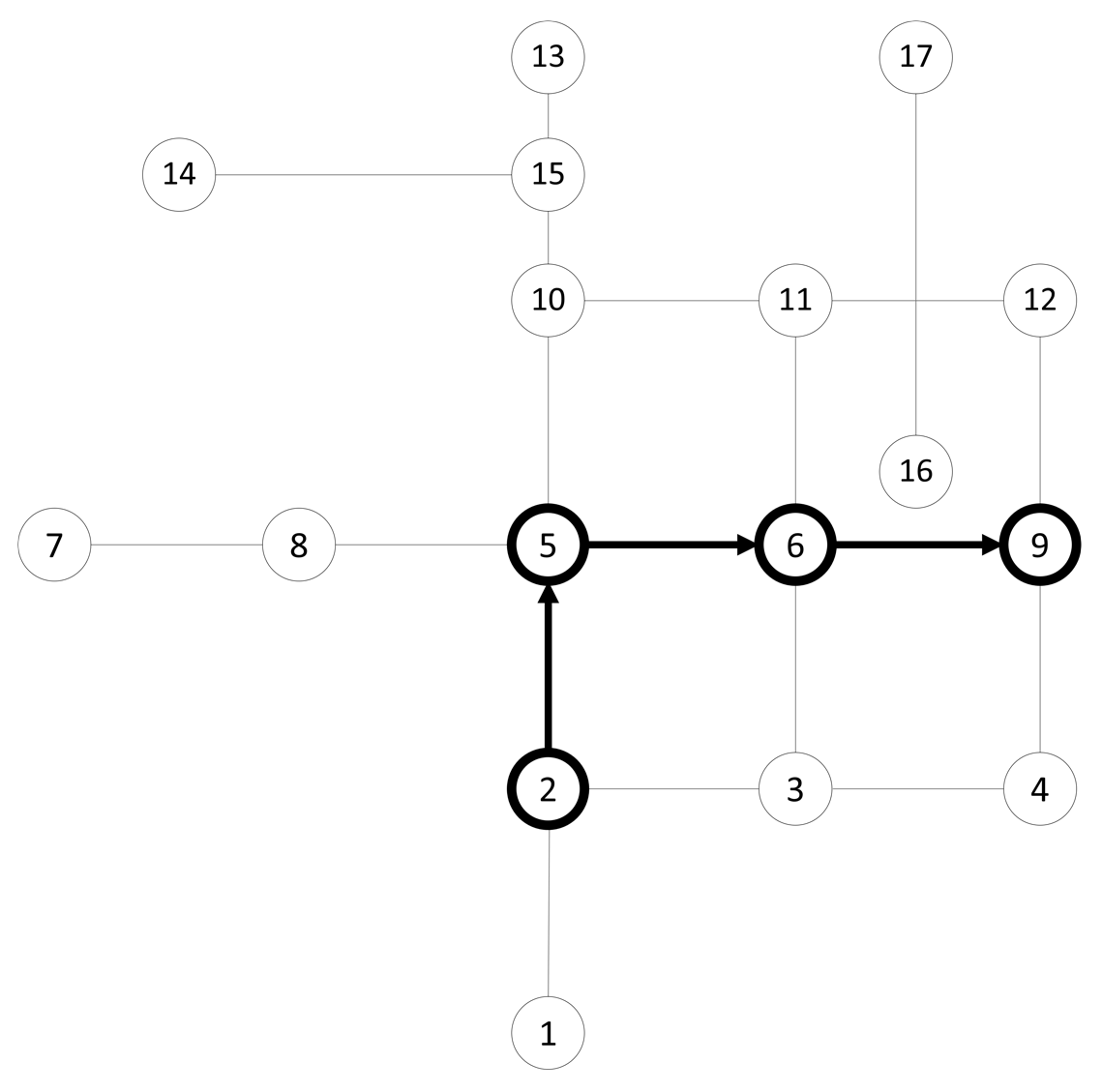
Now that the data is loaded, we can run a quick test. We'll use a simple algorithm called Dijkstra to calculate the shortest path from node 5 to node 12.

Dijkstra's algorithm is an effective and simple routing algorithm that runs a search on all available paths from point A to point B in a network, also known as the graph structure. It is not the most efficient routing algorithm, but will always find the best route. For more information on Dijkstra's algorithm, refer to Wikipedia, which has a good explanation, with illustrations, at http://en.wikipedia.org/wiki/Dijkstra%27s_algorithm. The animation at http://en.wikipedia.org/wiki/File:Dijkstras_progress_animation.gif is particularly helpful.

An important point to note is that the nodes created in pgRouting during the topology creation process are created unintentionally for some versions. This has been patched in future versions, but for some versions of pgRouting, this means that your node numbers will not be the same as those we use here in the book. View your data in an application to determine which nodes to use or whether you should use a k-nearest neighbors search for the node nearest to a static geographic point. See Chapter 11, Using Desktop Clients, for more information on viewing PostGIS data and Chapter 4, Working with Vector Data – Advanced Recipes, for approaches to finding the nearest node automatically:

SELECT * FROM pgr_dijkstra(
  'SELECT id, source, target, cost
  FROM chp06.edge_table_vertices_pgr', 2, 9,
);

The preceding query will result in the following:

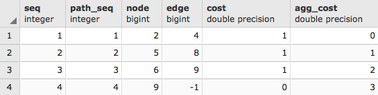
When we ask for a route using Dijkstra and other routing algorithms, the result often comes in the following form:

seq: This returns the sequence number so we can maintain the order of the output
node: This is the node ID
edge: This is the edge ID
cost: This is the cost for the route traversal (often, the distance)
agg_cost: This is the aggregated cost for the route from the starting node

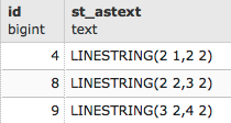
For example, to get the geometry back, we need to rejoin the edge IDs with the original table. To make this approach work transparently, we will use the WITH common table expression to create a temporary table to which we will join our geometry:

WITH dijkstra AS (
  SELECT pgr_dijkstra(
    'SELECT id, source, target, cost, x1, x2, y1, y2
    FROM chp06.edge_table', 2, 9
  )
)
SELECT id, ST_AsText(the_geom)
FROM chp06.edge_table et, dijkstra d
WHERE et.id = (d.pgr_dijkstra).edge;

The preceding code will give the following output:

Congratulations! You have just completed a route in pgRouting. The following diagram illustrates this scenario:

Table of Contents for
PostGIS Cookbook - Second Edition

How to do it...

Table of Contents for PostGIS Cookbook - Second Edition

Table of Contents for
PostGIS Cookbook - Second Edition