We will use the LiDAR data imported in the previous recipe as our dataset of choice. We named that table chp07.lidar. To perform a nearest-neighbor search, we will require an index created on the dataset. Spatial indexes, much like ordinary database table indexes, are similar to book indexes insofar as they help us find what we are looking for faster. Ordinarily, such an index-creation step would look like the following (which we won't run this time):

CREATE INDEX chp07_lidar_the_geom_idx  
ON chp07.lidar USING gist(the_geom); 

A 3D index does not perform as quickly as a 2D index for 2D queries, so a CREATE INDEX query defaults to creating a 2D index. In our case, we want to force the gist to apply to all three dimensions, so we will explicitly tell PostgreSQL to use the n-dimensional version of the index:

CREATE INDEX chp07_lidar_the_geom_3dx 
ON chp07.lidar USING gist(the_geom gist_geometry_ops_nd); 

Note that the approach depicted in the previous code would also work if we had a time dimension or a 3D plus time. Let's load a second 3D dataset and the stream centerlines that we will use in our query:

$ shp2pgsql -s 3734 -d -i -I -W LATIN1 -t 3DZ -g the_geom hydro_line chp07.hydro | PGPASSWORD=me psql -U me -d "postgis-cookbook" -h localhost  

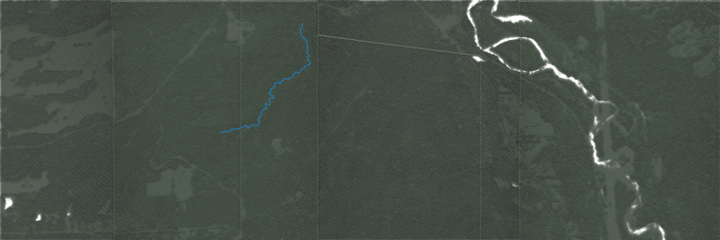
This data, as shown in the following image, overlays nicely with our LiDAR point cloud:

Now, we can build a simple query to retrieve all the LiDAR points within one foot of our stream centerline:

DROP TABLE IF EXISTS chp07.lidar_patches_within; 
CREATE TABLE chp07.lidar_patches_within AS 
SELECT chp07.lidar_patches.gid, chp07.lidar_patches.the_geom 
FROM chp07.lidar_patches, chp07.hydro  
WHERE ST_3DDWithin(chp07.hydro.the_geom, chp07.lidar_patches.the_geom, 5); 

But, this is a little bit of a sloppy approach; we could end up with duplicate LiDAR points, so we will refine our query with LEFT JOIN and SELECT DISTINCT instead, but continue using ST_DWithin as our limiting condition:

DROP TABLE IF EXISTS chp07.lidar_patches_within_distinct; 
CREATE TABLE chp07.lidar_patches_within_distinct AS 
SELECT DISTINCT (chp07.lidar_patches.the_geom), chp07.lidar_patches.gid  
FROM chp07.lidar_patches, chp07.hydro  
WHERE ST_3DDWithin(chp07.hydro.the_geom, chp07.lidar_patches.the_geom, 5); 

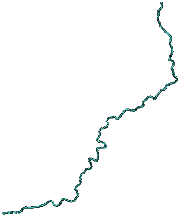
Now we can visualize our returned points, as shown in the following image:

Try this query using ST_DWithin instead of ST_3DDWithin. You'll find an interesting difference in the number of points returned, since ST_DWithin will collect LiDAR points that may be close to our streamline in the XY plane, but not as close when looking at a 3D distance.

You can imagine ST_3DWithin querying within a tunnel around our line. ST_DWithin, by contrast, is going to query a vertical wall of LiDAR points, as it is only searching for adjacent points based on XY distance, ignoring height altogether, and thus gathering up all the points within a narrow wall above and below our points.