Private information retrieval (PIR) LPPMs provide location privacy by mapping the spatial context to provide a private way to query a service without releasing any location information that could be obtained by third parties.

PIR-based methods can be classified as cryptography-based or hardware-based, according to [9]. Hardware-based methods use a special kind of secure coprocessor (SC) that acts as securely protected spaces in which the PIR query is processed in a non-decipherable way, as in [10]. Cryptography-based techniques only use logic resources, and do not require a special physical disposition on either the server or client-side.

In [10], the authors present a hybrid technique that uses a cloaking method through various-size grid Hilbert curves to limit the search domain of a generic cryptography-based PIR algorithm; however, the PIR processing on the database is still expensive, as shown in their experiments, and it is not practical for a user-defined level of privacy. This is because the method does not allow the cloaking grid cell size to be specified by the user, nor can it be changed once the whole grid has been calculated; in other words, no new PoIs can be added to the system. Other techniques can be found in [12].

PIR can also be combined with other techniques to increase the level of privacy. One type of compatible LPPM is the dummy query-based technique, where a set of random fake or dummy queries are generated for arbitrary locations within the greater search area (city, county, state, for example)  [13], [14]. The purpose of this is to hide the one that the user actually wants to send.

The main disadvantage of the dummy query technique is the overall cost of sending and processing a large number of requests for both the user and the server sides. In addition, one of the queries will contain the original exact location and point of interest of the user, so the original trajectory could still be traced based on the query records from a user - especially if no intelligence is applied when generating the dummies. There are improvements to this method discussed in [15], where rather than sending each point on a separate query, all the dummy and real locations are sent along with the location interest specified by the user. In [16], the authors propose a method to avoid the random generation of points for each iteration, which should reduce the possibility of detecting the trend in real points; but this technique requires a lot of resources from the device when generating trajectories for each dummy path, generates separate queries per path, and still reveals the user's location.

The LPPM presented as an example in this book is MaPIR – a Map-based PIR [17]. This is a method that applies a mapping technique to provide a common language for the user and server, and that is also capable of providing redundant answers to single queries without overhead on the server-side, which, in turn, can improve response time due to a reduction in its use of geographical queries.

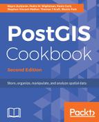
This technique creates a redundant geographical mapping of a certain area that uses the actual coordinate of the PoI to generate IDs on a different search scale. In the MaPIR paper, the decimal digit of the coordinate that will be used for the query. Near the Equator, each digit can be approximated to represent a certain distance, as shown in the following figure:

This can be generalized by saying that nearby locations will appear close at larger scales (closer to the integer portion of the location), but not necessarily in smaller ones. It could also show relatively far away points as though they were closer, if they share the same set of digits (nth digit of latitude and nth digit of longitude).

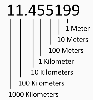
Once the digits have been obtained, depending on the selected scale, a mapping technique is needed to reduce the number to a single ID. On paper, a simple pseudo-random function is applied to reduce the two-dimensional domain to a one-dimensional one:

ID(Lat_Nth, Lon_Nth) = (((Lat_Nth + 1) * (Lon_Nth + 1)) mod p) - 1

In the preceding equation, we can see that p is the next prime number to the maximum desired ID. Given that for the paper the maximum ID was 9, the value of p is 11. After applying this function, the final map looks as follows:

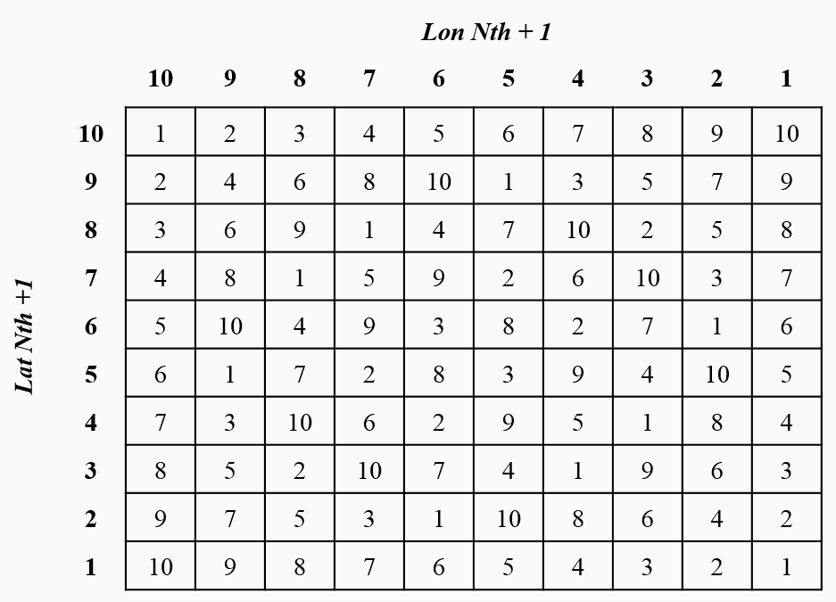
The following figure shows a sample PoI ID that represents a restaurant located at 10.964824,-74.804778. The final mapping grid cells will be 2, 6, and 1, using the scales k = 3, 2, and 1 respectively.

This information can be stored on a specific table in the database, or as the DBA determined best for the application:

Based on this structure, a query generated by a user will need to define the scale of search (within 100 m, 1 km, and so on), the type of business they are looking for, and the grid cell they are located. The server will receive the parameters and look for all restaurants in the same cell ID as the user. The results will return all restaurants located in the cells with the same ID, even if they are not close to the user. Given that cells are indistinguishable, an attacker that gains access to the server's log will only see that a user was in 1 of 10 cell IDs. Of course, some of the IDs may fall in inhabitable areas (such as in a forest or lake), but some level of redundancy will always be present.