Paths can also have curves. The concept is still the same; you connect several data points with lines. The main difference is that now you apply a curve to each line as it connects the dots. There are three types of curve commands:

• Cubic Bézier
• Quadratic Bézier
• Elliptical arc

Each command is explained in detail at http://www.w3.org/TR/SVG11/paths.html. As an example, let's apply a cubic Bézier curve to the triangle. The format for the command is as follows:

C x1 y1 x2 y2 x y 

This command can be inserted into the path structure at any point:

• C: Indicates that we are applying a Cubic Bézier curve, just as L in the previous example indicates a straight line
• x1 and y1: Adds a control point to influence the curve's tangent
• x2 and y2: Adds a second control point after applying x1 and y1
• x and y: Indicates the final resting place of the line

To apply this command to our previous triangle, we need to replace the second line command (320 120) with a cubic command (C 200 70 480 290 320 120).

Before, the statement was as follows:

<path d="M 120 120 L 220 220, 320 120 Z"></path> 

After adding the cubic command, it will be as follows:

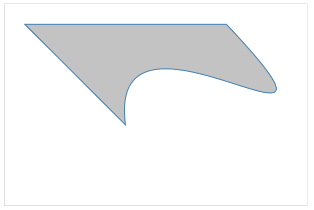
<path d="M 120 120 L 220 220, C 200 70 480 290 320 120 Z"></path> 

This will produce the following shape:

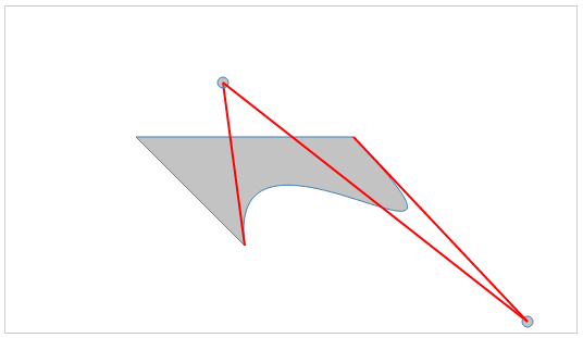
To illustrate how the cubic Bézier curve works, let's draw circles and lines to show the control points in the C command:

<svg  height="300" width="525"> 
      <path d="M 120 120 L 220 220 C 200 70 480 290 320 120 Z ">
       </path> 
      <line x1="220"  y1="220" x2="200" y2="70"></line> 
      <circle cx="200" cy="70" r="5" ></circle> 
      <line x1="200"  y1="70"  x2="480" y2="290"></line> 
      <circle cx="480" cy="290"  r="5"></circle> 
      <line x1="480"  y1="290" x2="320" y2="120"></line> 
</svg> 

The output should look like the one shown in the following screenshot, and can be experimented with at http://localhost:8080/chapter-2/curves.html. You can see the angles created by the control points (indicated by circles in the output) and the cubic Bézier curves applied.

SVG paths are the main tool leveraged when drawing geographic regions. However, imagine if you were to draw an entire map by hand using SVG paths; the task would become exhausting! For example, the command structure for the map of Europe in our first chapter has 3,366,121 characters in it! Even a simple state such as Colorado would be a lot of code if executed by hand:

<path xmlns="http://www.w3.org/2000/svg" id="CO_1_" 
 style="fill:#ff0000" d="M 115.25800,104.81000 L 
 116.51200,84.744000 L 117.00000,77.915000 L 106.82700,77.077000 L 
 99.371000,76.452000 L 88.014000,75.198000 L 81.709000,74.431000 L 
 80.907000,81.189000 L 79.932000,88.018000 L 78.788000,96.547000 L 
 78.329000,99.932000 L 78.154000,101.11800 L 88.641000,102.37200 L 
 99.898000,103.72200 L 109.88400,104.39200 L 111.91300,104.60300 L 
 115.39700,104.77700"/>

We will learn in later chapters how D3 will come to the rescue.